Digitizing and approximating graphs of functions using Wolfram Mathematica and Graph Digitizer
The task of digitizing graphs of functions and curves has to face almost every engineer and student. The traditional "manual" method is very inconvenient and also introduces large errors in the data. For a one-time task, this method is not so bad, but if there are more than one graphs and each one contains not one curve, but a family of curves?
In the process of carrying out laboratory practical work in physics, I often have the task of determining the value of a function from its graph presented on paper, for further calculations. Since the processing of such graphs on a computer significantly increases the speed and accuracy of this process, it was decided to explore the possibilities for digitizing the graph and building a mathematical model of the curve presented on the graph.
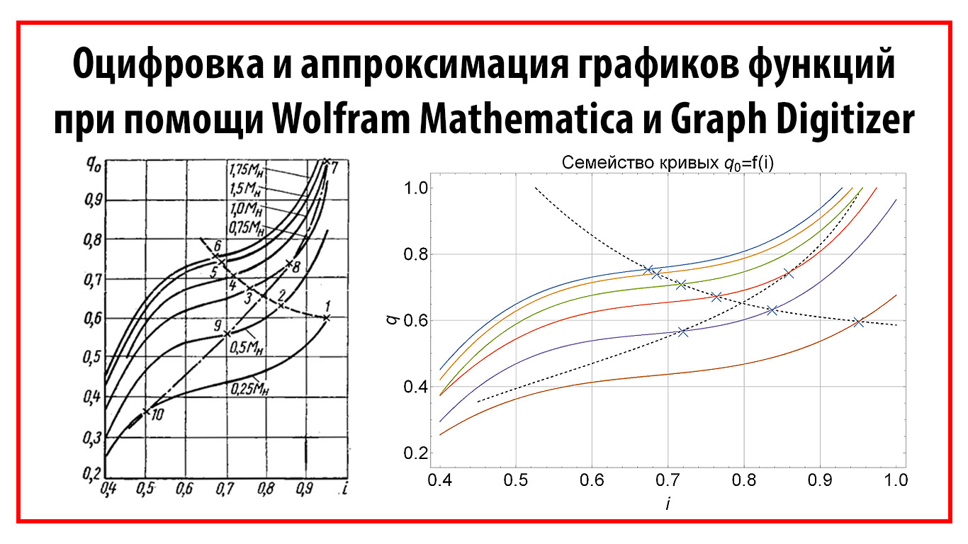
As an example, I took a graph of the efficiency of the generator from its power from a laboratory workshop on electrical engineering. During the execution of the work, I performed a scan of the graph, image processing of the graph, digitization of coordinates and the construction of a mathematical model of the curve.
')
After scanning, the first thing to do is to bring the resulting image to full contrast and align one of the axes of the graph. Next, you need to increase the sharpness and resize the image. If the size and resolution are too large, difficulties arise at the subsequent stages of work.
Image processing, I recommend the program Adobe Photoshop. Using the Curves tool, we achieve a full-fledged contrast, then use the Smart Sharpen filter to increase sharpness. The undoubted advantage of Photoshop is the ability to process a large number of images by recording the action (Action) and applying it in conjunction with batch processing (File - batch processing).
To speed up the process, the processing can be performed in the scanning program using pre-prepared presets or automatic algorithms.

Figure 1.1 - Graphic image Before processing and After processing
To digitize coordinates, I used the shareware program GetData Graph Digitize version 2.26. After starting the program, open our processed image "File - Open Image". After opening, we will see a standard workspace.
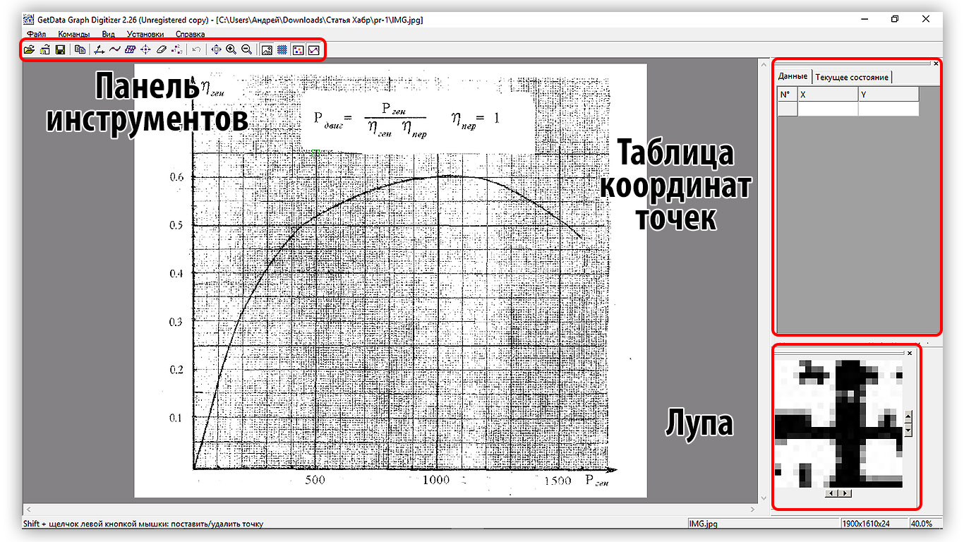
Figure 2.1 - Standard Graph Digitize Interface
The first thing we need to do is to establish a coordinate system, i.e. mark the lines of the axes. To do this, go to "Commands - Set the coordinate system." Further, holding the LMB, we find the point of origin and click on it. In the window that appears, enter the value of the origin (Xmin). Next, set the values Xmax, Ymin and Ymax in the same way. For convenient installation of points it is necessary to open the “View - Magnifier” magnifying glass window. After the control points are set, the axis lines appear and the "Coordinate System Parameters" window opens in which you can reassign the values of the control points and set the logarithmic axis scale.
For visual quality control of the SC installation, you can display the grid with the specified step “View - Show grid”. In case of correct installation of the IC, the grid lines should be strictly parallel to the lines in the image of the graph. It should be noted that when scanning turns, the graph often turns out to be in the bend area, and one of the axes turns out to be bent. In this case, it is not possible to set the CS correctly, therefore at the scanning stage it is necessary to press the turn to the glass more tightly.

Figure 2.2 - View with the established coordinate system and grid
Let's start installing points on the chart. To do this, go to the point setting mode (Ctrl + P). In this mode, click LMB to set a new point. To display the table of coordinates of the selected points, go to the “View - Information Window”. To delete points, use the data point eraser “Commands - Data Eraser” (Ctrl + E)
In my experience, a greater number of points must be installed in the vicinity of the inflection points of the curve; on the linear sections of the curve, it can be limited to a small number of them.
If there is more than 1 curve or a family of curves on the graph, then after setting the points on the first one, you need to add a new line “Commands - Add Line”. Then it will be possible to set points on the second curve, etc.
If there is no grid on the graph image, then you can use the automatic curve trace algorithm (Ctrl + T). In the presence of a grid, the algorithm gives a lot of errors.
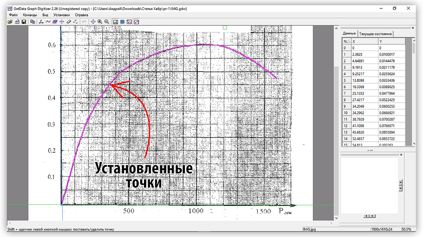
Figure 2.3 - View with set points on the curve
For further processing of the data, it is necessary to export the coordinates of the points to a .txt file or to the clipboard (conveniently if we have only one curve). In the GetData Graph Digitize program, export to .txt is performed by calling the “File - Data Export” command (Ctrl + Alt + E). After clicking in the window that opens, you are prompted to set the save path and file name.
In the “Settings - Parameters” menu the output format is set. You can also enable sorting points by the value of the X coordinate, if a unique Y exists on your curve for each X, to eliminate random errors in the sequence of setting points.

Figure 2.4 - Export Settings
In the final, we will perform an approximation of the obtained data and verify the correctness of the obtained mathematical model. For this, I propose to use the computer algebra system Wolfram Mathematica.
To quickly import data into Wolfram Mathematica, copy the coordinates of points from the exported file and paste it into an empty Excel cell. As a result, 2 columns of data X and Y will appear on the sheet, respectively.
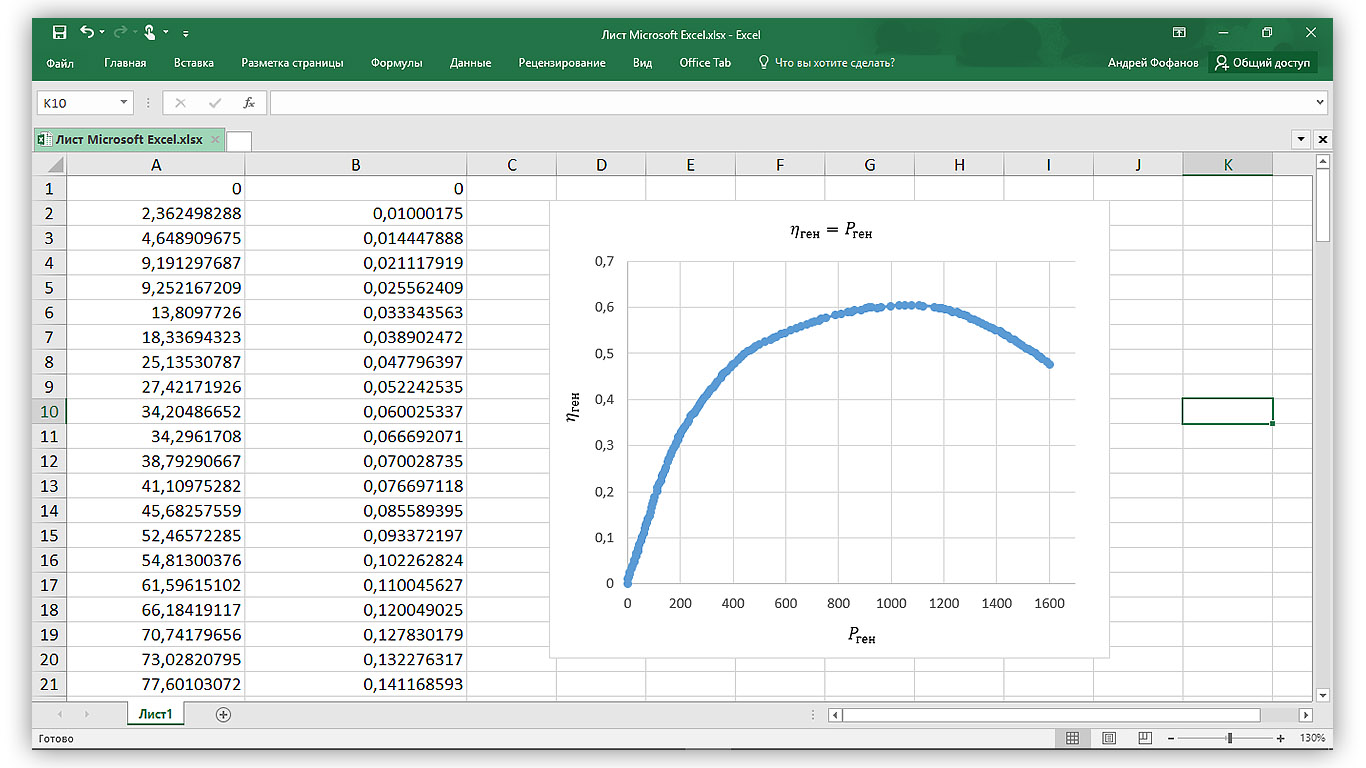
Figure 3.1 - Data in Excel
The next step is to create a new Wolfram Mathematica document and drag the Excel file into it. The result is a list of lists containing the coordinates of the points. Give it the variable data.
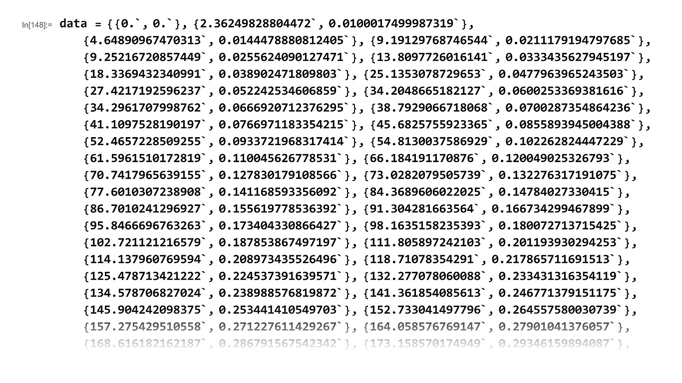
Figure 3.2 - Imported data in Wolfram Mathematica
Display the imported data using the ListPlot [] function.

Figure 3.3 - Graphic display of points in the form of a scatter diagram
Approximate the points by a polynomial of degree 5. For this we use the function LinearModelFit []. As a result, we get an object of class FittedModel []. Give it the fit variable.
We calculate the coefficient of determination R ^ 2, which shows how much of the variation (spread) of the variable explains the resulting equation. The closer this coefficient is to unity, the greater the proportion of variation that explains the equation. To do this, we specify “RSquared” as the argument of the fit function. In this case, R ^ 2 = 0.99, which means that our model explains 99.9% of the variation of the variable.
To calculate the Y value, it is necessary to specify the required X value as an argument to the fit function.
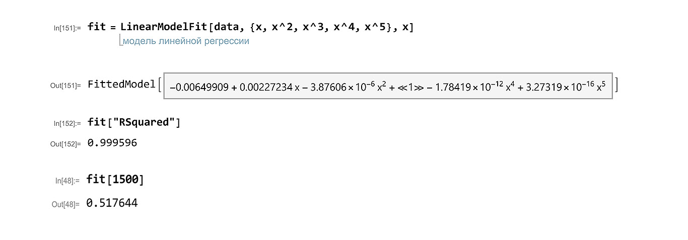
Figure 3.4 - Approximation of points, calculation of the coefficient of determination and calculation of the function value
In addition to calculating the coefficient of determination, we will conduct a regression analysis. This time, the argument of the fit function is “ANOVATable”. According to the obtained result, it can be argued that the use of each term of the approximating polynomial is justified. Let's display the resulting equation explicitly, for this we apply the function Normal [] to the fit variable.

Figure 3.5 - Regression analysis and the polynom explicitly
Next, we construct a graph of the polynomial and display the initial points on it. Using the standard syntax, set the style of the chart and add labels to the axes and the name of the chart.

Figure 3.6 - Final Schedule
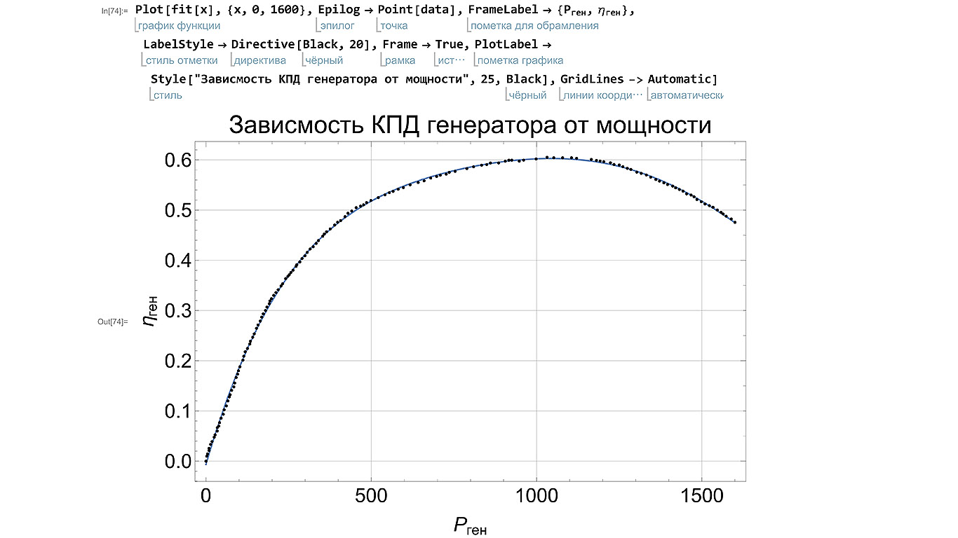
Figure 3.7 - Comparison of the final schedule with the original data
The possibilities for analyzing the mathematical model in Wolfram Mathematica are truly enormous, but we will limit ourselves to those presented above. Interested parties can learn more by calculating the fit ["Properties"] function.
Conclusion:
As a result, we studied the possibility of using Wolfram Mathematica and Graph Digitizer for digitizing graphs and selecting a mathematical model of the curve. The software used allows you to complete the task with minimal effort and with high quality.
PS: In the comments you can briefly tell how often you have to deal with a similar task in your activity? I will be glad to answer questions.
In the process of carrying out laboratory practical work in physics, I often have the task of determining the value of a function from its graph presented on paper, for further calculations. Since the processing of such graphs on a computer significantly increases the speed and accuracy of this process, it was decided to explore the possibilities for digitizing the graph and building a mathematical model of the curve presented on the graph.
As an example, I took a graph of the efficiency of the generator from its power from a laboratory workshop on electrical engineering. During the execution of the work, I performed a scan of the graph, image processing of the graph, digitization of coordinates and the construction of a mathematical model of the curve.
')
1. Image preparation
After scanning, the first thing to do is to bring the resulting image to full contrast and align one of the axes of the graph. Next, you need to increase the sharpness and resize the image. If the size and resolution are too large, difficulties arise at the subsequent stages of work.
Image processing, I recommend the program Adobe Photoshop. Using the Curves tool, we achieve a full-fledged contrast, then use the Smart Sharpen filter to increase sharpness. The undoubted advantage of Photoshop is the ability to process a large number of images by recording the action (Action) and applying it in conjunction with batch processing (File - batch processing).
To speed up the process, the processing can be performed in the scanning program using pre-prepared presets or automatic algorithms.
Figure 1.1 - Graphic image Before processing and After processing
2. Digitization of coordinates
To digitize coordinates, I used the shareware program GetData Graph Digitize version 2.26. After starting the program, open our processed image "File - Open Image". After opening, we will see a standard workspace.
Figure 2.1 - Standard Graph Digitize Interface
2.1. Setting the coordinate system (SC)
The first thing we need to do is to establish a coordinate system, i.e. mark the lines of the axes. To do this, go to "Commands - Set the coordinate system." Further, holding the LMB, we find the point of origin and click on it. In the window that appears, enter the value of the origin (Xmin). Next, set the values Xmax, Ymin and Ymax in the same way. For convenient installation of points it is necessary to open the “View - Magnifier” magnifying glass window. After the control points are set, the axis lines appear and the "Coordinate System Parameters" window opens in which you can reassign the values of the control points and set the logarithmic axis scale.
For visual quality control of the SC installation, you can display the grid with the specified step “View - Show grid”. In case of correct installation of the IC, the grid lines should be strictly parallel to the lines in the image of the graph. It should be noted that when scanning turns, the graph often turns out to be in the bend area, and one of the axes turns out to be bent. In this case, it is not possible to set the CS correctly, therefore at the scanning stage it is necessary to press the turn to the glass more tightly.
Figure 2.2 - View with the established coordinate system and grid
2.3. Curve digitization
Let's start installing points on the chart. To do this, go to the point setting mode (Ctrl + P). In this mode, click LMB to set a new point. To display the table of coordinates of the selected points, go to the “View - Information Window”. To delete points, use the data point eraser “Commands - Data Eraser” (Ctrl + E)
In my experience, a greater number of points must be installed in the vicinity of the inflection points of the curve; on the linear sections of the curve, it can be limited to a small number of them.
If there is more than 1 curve or a family of curves on the graph, then after setting the points on the first one, you need to add a new line “Commands - Add Line”. Then it will be possible to set points on the second curve, etc.
If there is no grid on the graph image, then you can use the automatic curve trace algorithm (Ctrl + T). In the presence of a grid, the algorithm gives a lot of errors.
Figure 2.3 - View with set points on the curve
2.4. Data export
For further processing of the data, it is necessary to export the coordinates of the points to a .txt file or to the clipboard (conveniently if we have only one curve). In the GetData Graph Digitize program, export to .txt is performed by calling the “File - Data Export” command (Ctrl + Alt + E). After clicking in the window that opens, you are prompted to set the save path and file name.
File with exported data
Created by GetData Graph Digitizer 2.26.0.20, created on October 01 2017, 21:16,
based on the file 'C: \ Users \ Andrey \ Downloads \ Article Habr \ pr-1 \ IMG.jpg'
Line # 1
0.00000000000000 0.00000000000000
2.36249828804472 0.0100017499987319
4.64890967470313 0.0144478880812405
9.19129768746544 0.0211179194797685
9.25216720857449 0.0255624090127471
13.8097726016141 0.0333435627945197
18.3369432340991 0.0389024718098030
25.1353078729653 0.0477963965243503
27.4217192596237 0.0522425346068590
34.2048665182127 0.0600253369381616
34.2961707998762 0.0666920712376295
38.7929066718068 0.0700287354864236
41.1097528190197 0.0766971183354215
45.6825755923365 0.0855893945004388
52.4657228509255 0.0933721968317414
54.8130037586929 0.102262824447229
61.5961510172819 0.110045626778531
66.1841911708760 0.120049025326793
70.7417965639155 0.127830179108566
73.0282079505739 0.132276317191075
77.6010307238908 0.141168593356092
84.3689606022025 0.147840273304150
86.7010241296927 0.155619778536392
91.3042816635640 0.166734299467899
95.8466696763263 0.173404330866427
98.1635158235393 0.180072713715425
102.721121216579 0.187853867497197
111.805897242103 0.201193930294253
114.137960769594 0.208973435526496
118.710783542910 0.217865711691513
125.478713421222 0.224537391639571
132.277078060088 0.233431316354119
134.578706827024 0.238988576819872
141.361854085613 0.246771379151175
145.904242098375 0.253441410549703
152.733041497796 0.264557580030739
157.275429510558 0.271227611429267
164.058576769147 0.279010413760570
168.616182162187 0.286791567542342
173.158570174949 0.293461598940870
179.926500053261 0.300133278888928
184.468888066023 0.306803310287456
191.236817944335 0.313474990235514
193.538446711271 0.319032250701268
198.050399963478 0.323480037333306
204.818329841790 0.330151717281364
211.571042339824 0.335712274846178
218.323754837859 0.341272832410991
227.332443961997 0.349057283291824
231.844397214205 0.353505069923862
240.883521098898 0.363511765571184
247.621016216655 0.367961200752753
252.117752088585 0.371297865001547
256.629705340793 0.375745651633586
263.367200458550 0.380195086815154
272.375889582689 0.387979537695987
274.647083589070 0.391314553395251
283.625337952654 0.396876759509595
290.393267830965 0.403548439457653
299.371522194549 0.409110645571996
306.139452072861 0.415782325520054
315.132923816722 0.422455654017642
324.095960800028 0.426906737748741
333.089432543889 0.433580066246329
339.842145041924 0.439140623811142
353.317135277438 0.448039494174280
357.829088529646 0.452487280806318
364.566583647403 0.456936715987887
375.770379876536 0.462500570651760
389.230152731773 0.470288318631653
398.208407095357 0.475850524745997
407.156226698386 0.479190486093851
420.615999553624 0.486978234073743
429.609471297485 0.493651562571331
440.798050146340 0.498104294851960
454.242605621300 0.504780920448608
467.641508955428 0.508124178895523
476.574111178180 0.510353017860132
485.537148161487 0.514804101591231
498.951268875892 0.519258482421390
521.282774432772 0.524830579832913
541.388738124103 0.530401028694907
554.802858838508 0.534855409525066
565.961002926809 0.537085897039205
581.600665506764 0.541541926418894
597.225110706442 0.544886833415338
617.331074397772 0.550457282277332
641.872904439924 0.554919905855141
659.722891505151 0.558266461401115
679.828855196482 0.563836910263109
697.678842261709 0.567183465809083
708.836986350010 0.569413953323222
726.671756034959 0.571649386485952
735.619575637989 0.574989347833806
753.454345322938 0.577224780996536
789.139102073114 0.582806769705239
809.214631003891 0.586154973800744
833.741243665765 0.589506474995308
849.335254104888 0.590629137225263
860.508615573467 0.593970747122647
884.989576094510 0.593988881167477
905.065105025286 0.597337085262982
916.223249113588 0.599567572777121
925.125416575785 0.599574166975241
947.350400470724 0.597368407704052
960.734086424575 0.599600543767722
998.598732899469 0.601850813876222
1032.02751302354 0.605208909268906
1052.04217243321 0.604112623831432
1078.74867481980 0.604132406425792
1105.45517720639 0.604152189020153
1121.01875288496 0.603052606483618
1165.49915543539 0.600863332707730
1181.04751373369 0.598652627787951
1192.16000568116 0.597549748152356
1203.27249762862 0.596446868516762
1223.27193965801 0.594239460696043
1234.35399684493 0.590914336293959
1249.91757252350 0.589814753757425
1260.99962971041 0.586489629355341
1274.30722876288 0.583166153502787
1285.40450333007 0.580952151483948
1303.13275135308 0.575409727963965
1316.45556778582 0.573197374494656
1331.98870870383 0.569875547191632
1345.28109037602 0.565440948955834
1360.79901391376 0.561007999269566
1371.88107110067 0.557682874867482
1385.18867015314 0.554359399014928
1396.27072734005 0.551034274612844
1411.80386825807 0.547712447309821
1420.66038357943 0.544385674358207
1431.74244076635 0.541060549956123
1442.82449795326 0.537735425554039
1453.87612037962 0.532188056385466
1467.19893681236 0.529975702916157
1476.05545213373 0.526648929964543
1484.88153269454 0.521099912246440
1498.17391436673 0.516665314010642
1509.24075417337 0.512229067225314
1522.54835322583 0.508905591372760
1533.63041041275 0.505580466970676
1546.90757470466 0.500034746351633
1557.97441451129 0.495598499566305
1564.60538796711 0.492270078065161
1573.44668590820 0.487832182730302
1588.94939206566 0.482288110660789
1599.98579711174 0.475629619108972
In the “Settings - Parameters” menu the output format is set. You can also enable sorting points by the value of the X coordinate, if a unique Y exists on your curve for each X, to eliminate random errors in the sequence of setting points.
Figure 2.4 - Export Settings
3. Construction of a mathematical model of the curve
In the final, we will perform an approximation of the obtained data and verify the correctness of the obtained mathematical model. For this, I propose to use the computer algebra system Wolfram Mathematica.
To quickly import data into Wolfram Mathematica, copy the coordinates of points from the exported file and paste it into an empty Excel cell. As a result, 2 columns of data X and Y will appear on the sheet, respectively.
Figure 3.1 - Data in Excel
The next step is to create a new Wolfram Mathematica document and drag the Excel file into it. The result is a list of lists containing the coordinates of the points. Give it the variable data.
Figure 3.2 - Imported data in Wolfram Mathematica
Display the imported data using the ListPlot [] function.
Figure 3.3 - Graphic display of points in the form of a scatter diagram
Approximate the points by a polynomial of degree 5. For this we use the function LinearModelFit []. As a result, we get an object of class FittedModel []. Give it the fit variable.
We calculate the coefficient of determination R ^ 2, which shows how much of the variation (spread) of the variable explains the resulting equation. The closer this coefficient is to unity, the greater the proportion of variation that explains the equation. To do this, we specify “RSquared” as the argument of the fit function. In this case, R ^ 2 = 0.99, which means that our model explains 99.9% of the variation of the variable.
To calculate the Y value, it is necessary to specify the required X value as an argument to the fit function.
Figure 3.4 - Approximation of points, calculation of the coefficient of determination and calculation of the function value
In addition to calculating the coefficient of determination, we will conduct a regression analysis. This time, the argument of the fit function is “ANOVATable”. According to the obtained result, it can be argued that the use of each term of the approximating polynomial is justified. Let's display the resulting equation explicitly, for this we apply the function Normal [] to the fit variable.
Figure 3.5 - Regression analysis and the polynom explicitly
Next, we construct a graph of the polynomial and display the initial points on it. Using the standard syntax, set the style of the chart and add labels to the axes and the name of the chart.
Figure 3.6 - Final Schedule
Figure 3.7 - Comparison of the final schedule with the original data
The possibilities for analyzing the mathematical model in Wolfram Mathematica are truly enormous, but we will limit ourselves to those presented above. Interested parties can learn more by calculating the fit ["Properties"] function.
Conclusion:
As a result, we studied the possibility of using Wolfram Mathematica and Graph Digitizer for digitizing graphs and selecting a mathematical model of the curve. The software used allows you to complete the task with minimal effort and with high quality.
PS: In the comments you can briefly tell how often you have to deal with a similar task in your activity? I will be glad to answer questions.
Source: https://habr.com/ru/post/339332/
All Articles