Identify hidden data dependencies to improve the quality of the forecast in machine learning

Article layout

1. Formulation of the problem.
2. Formal description of the task.
3. Examples of tasks.
4. A few examples on synthetic data with hidden linear dependencies.
5. What other hidden dependencies may be contained in the data.
6. Automation of dependency search.

• The number of signs is less than the threshold value.
• The number of signs exceeds the threshold value.

Formulation of the problem

Often in machine learning there are situations when data are collected a priori, and only then there is a need to divide a certain sample into known classes. As a consequence, a situation may often arise when the existing set of features is poorly suited for effective classification. At least at the first approximation.

In such a situation, it is possible to build compositions of poorly working separately methods, or you can start with enriching the data by identifying hidden dependencies between the features. And then build on the basis of the dependencies found new sets of features, some of which can potentially give a significant increase in the quality of classification.

Formal task description

We are faced with the task of classifying L objects defined by n real numbers. We will consider a simple two-class case when the class labels are −1 and +1. Our goal is to build a linear classifier, that is, a function that returns −1 or + 1. At the same time, the set of feature descriptions is such that the hypothesis of compactness does not work for objects of opposite classes, measured on a given set of features, and the dividing hyperplane is extremely ineffective.
')
In other words, it looks as if the classification problem on a given set of objects cannot be solved effectively.

So, we have a column of answers containing the numbers -1 or 1, and the corresponding matrix of values ​​of attributes X1 ... Xn, consisting of L rows and n columns.

We set ourselves a subtask to find such dependencies F (Xi, Xj) that could act as new features for classified objects and help us build the optimal classifier.

Examples of tasks

Let's look at our task of finding the functions F (Xi, Xj) with examples. Of course, very vital.

Examples will be associated with leprechauns. Leprechauns, if someone does not know, exist somewhere near us, even though almost no one has seen them. And they, like people, have their computers, the Internet and social networks. Most of the time they devote to finding gold and storing it in their bags. However, in addition to honest leprechauns, there are those who are trying to distance themselves from this important work. They are called leprechauns dissidents. And precisely because of them the rate of increase in the volume of gold in leprechauns can not reach the desired value!

Since in the world of leprechauns there is also machine learning, they have learned to find them based on their behavior in large social networks. But there is a problem! Every year there are a lot of young social networks trying to capture the market, but still not able to collect enough data about their users for analysis! And the data that they collect is not enough to distinguish a decent leprechaun from a dissident leprechaun! And here we are faced with the need to look for hidden dependencies in the existing feature descriptions in order to be able to build an optimal classifier on the basis of data that are insufficient at first glance.

However, the example of social networks will probably be too difficult to parse, so let's try to solve a similar problem using the example of nuclear leprechaun processors. They are characterized by 4 main features:

a) Reactor Rotation Speed ​​(ppm)
b) Computational power (trl calculations / sec)
c) The speed of rotation of the reactor under load (ppm) and
d) Computational power under load (trillion calculations / sec)

Nuclear processors are produced by 2 main firms: 0 and 1 ('Black Zero' and 'The First'). In this case, Black Zero prices are twice as low, but the resource is also five times lower! However, the main state. The supplier of nuclear processors is constantly trying to deceive the customer and, instead of paying for The First machines, deliver cheaper and less reliable Black Zero machines. At the same time, the variation of the operating parameters of the reactors is so great that it is impossible to distinguish one from the other by the main characteristics for most measurements. Table 1 shows the characteristics of 50 randomly selected machines for each of the firms:


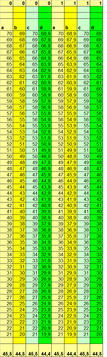
Table 1

For ease of comparison, objects of classes 1 and 0 are located not vertically, but laterally relative to each other. In the above example, it can be seen that, in general, the computing power parameters depend on the reactor speed, and, for machines from different manufacturers, depend somewhat differently: for Black Zero machines, compared to The First machines, the number of calculations is higher under normal conditions for similar reactor speeds, but lower under load. Of course, this is because The First machines without a load enter into the plasma saving mode, resulting in a slight decrease in performance. But under load, they are clearly ahead of the competitor.

But we see this dependence, because the data are specially selected so that this dependence is visible. In reality, among many thousands of dimensions and dozens (if not hundreds) of signs that cannot be so beautifully sorted as in this fictitious example, it is usually simply impossible to see with such eyes the dependencies. And if the whole business specificity of each attribute is still not completely clear, then trying to find such regularities with your eyes is at least an inefficient task.

Therefore, while moving within the paradigm of automating the learning of an algorithm, we would like to exclude to the maximum the human factor from the process of finding the dependencies between the signs. Let's look at several options for hidden dependencies and think about how best to organize the process of their detection.

Some examples on synthetic data with hidden linear dependencies

Option dependency 1. Xj = K * Xi + C, K = 1

The first variant of dependence says: the j-th feature of the object is linearly dependent on the i-th feature, as well as on the free term represented by a constant.
In our narrow example, the proportionality coefficient will be equal to one, so that you can better see the contribution of the free term.

Let b = a - 1, d = c - 1.1 for class 0 and vice versa for class 1 (b = a - 1.1, d = c - 1)

In this case, of course, it’s obvious that a new column with values
(d - b)
will give for the objects of the 0th and 1st classes, respectively
(c - 1.1) - (a - 1) = c - a - 0.1
and
(c - 1) - (a - 1.1) = c - a + 0.1
respectively. And this, in turn, with the homogeneity of the data in columns A and C (and this is one of the conditions in our problem), gives us a good tool for separating objects. And at a minimum we can count on the positive contribution of this new column to the final classification.

The result of such a calculation on our invented data you can see in Table 2:


table 2

This situation, despite the apparent artificiality, actually takes place in life. An example is the need to implement a certain condition to perform a series of regulated actions that have a constant set of side effects. In the case of nuclear processors in our example, the constant degradation of computational power may be associated with the need to start a fixed process to get to work under load. In life, the launch of an additional generator, a fixed allocation of resources to the reserve, energy to start the internal combustion engine or an industrial generator at thermal power plants, etc.

However, the choice of this particular function F (d, b) in the real problem will certainly not be obvious. Therefore, let's consider for a start, to what results a different choice of F (Xi, Xj) will lead us

F(Xi, Xj) = Xi/Xj

Speaking in terms of the characteristics of our problem, here we can try to measure, for example, the degradation of computational power under load (B / D). Moreover, on the assumption that such a degradation does not depend on a constant, but is completely relative value.
Let's see what happens as a result.


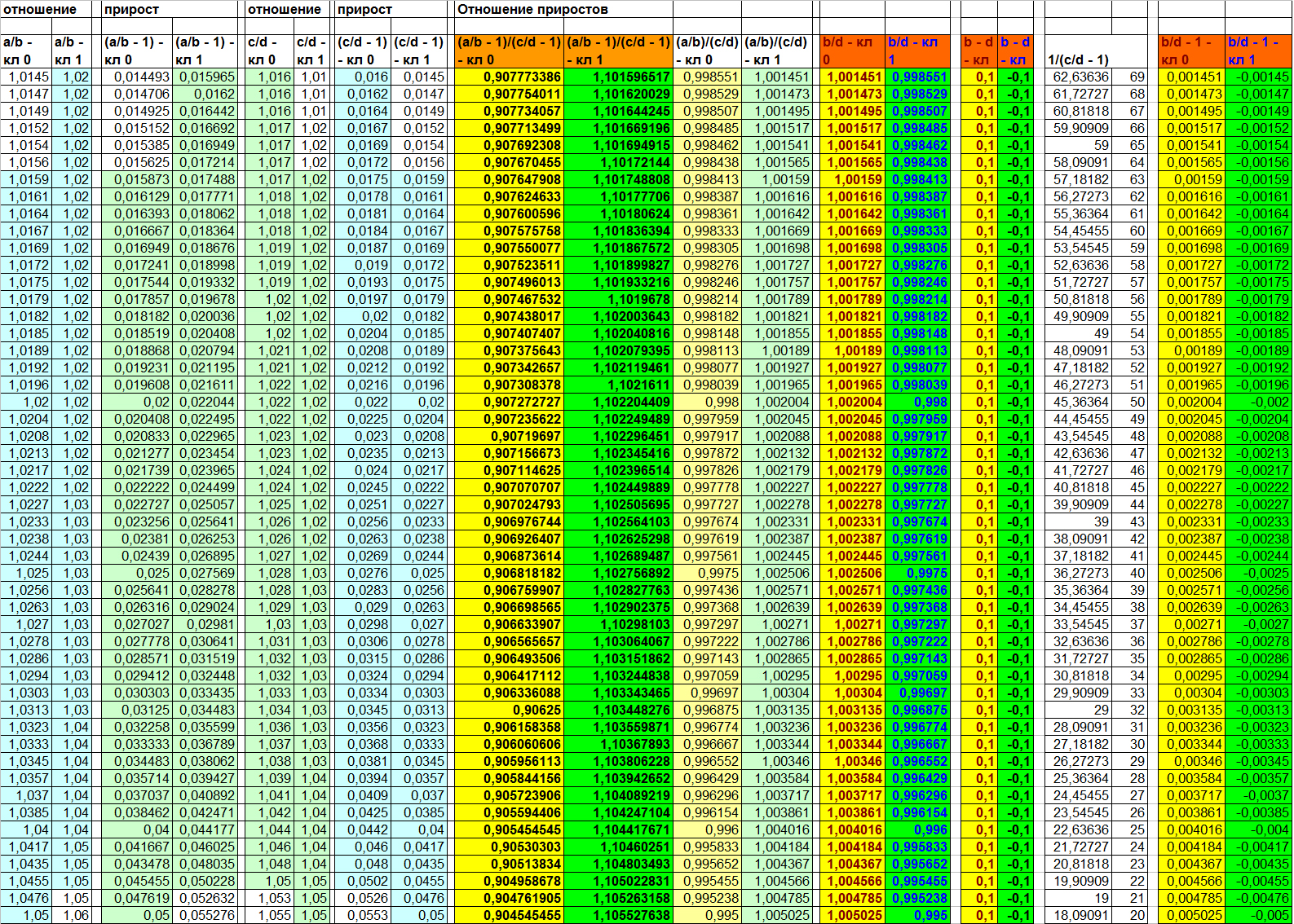
Table 3

As can be seen in Table 3, the relations (A / B) and (C / D) are not informative. Objects of opposite classes on them are still strongly mixed. But the B / D ratio is expected to make the sample linearly separable. Just like in the case of (B - D). However, running a little ahead, I will say that the reason for this linear separability on a given basis is still somewhat different than for the difference function. This will be clearly seen in the following example.

In the meantime, let's omit this nuance and think about what might be wrong with this version of the dependency. For the algorithm, most likely nothing. But for a person the visual signs for both classes may seem very close. Of course, in this example, all the values ​​are beautifully distributed on opposite sides of the unit, but in the life of such clarity may not be. How to solve this cosmetic problem? One of the simplest options is to calculate the increment in the numerator relative to the magnitude of the value in the denominator. What does it mean?

Calculating the ratio (X / Y), we get the answer to the question "How many times will Y fit in the value of X". However, it is sometimes more profitable to solve the question “How many Y's should be added to the value of Y in order to get X”. In the second case, we are looking for growth. Growth can be positive and negative and is expressed by a simple formula (X / Y - 1). Minus one - because we take one Y per unit of measurement.

Let's look again at table 3 (into the two rightmost columns) and pay attention to the fact that now we clearly see that the increment for objects of different classes is the value of the same sign. Therefore, we can talk about the different directions of growth of B from D for different classes. And it is precisely this factor that in this case actually plays the key role in the fact that the attribute (B / D) makes the sample linearly separable. Conclusion: each of the functions: (B - D) and (B / D) (or B / D - 1) makes the sample linearly separable in a slightly different way, which means that there may be situations where only one of them will be productive for some pair of symptoms . But more on this in more detail later. Now let's move on to the third function - the last one for the first example.

(A / B) / (C / D) - linear relationship
or
(A / B - 1) / (C / D - 1) - increment ratio

What can cause us to consider linear relationships or growth relations? In our example of two different equipment manufacturers, such a calculation has the following meaning: “how much will the dependence of performance on turns change when the load is connected”.

Well, quite a legitimate question. Given that we are talking about different manufacturers, different behavior of equipment with increasing load is quite expected. In life situations, we can talk about the fact that there are two relationships: F (Xi, Xj) and F (Xii, Xjj), and each of them is actually a function of a set of parameters unknown to us: F (M) and F '(M). And if such a hypothesis is correct, we can assume that even if each of the functions F and F 'manifests itself equally for objects of different classes, their composition F "(F, F') may manifest differently on objects of different classes, since In reality, these different classes have significantly different parameters unknown to us from the set M.

In our example, of course, we initially know where the legs of this second-order relationship grow from, since they themselves compiled the data accordingly. In life, however, we may not know this and rely only on the fact that such a relationship exists. And therefore try to find it.

Let's go back to table 3 (four central columns) and see how these functions manifest themselves for pairs (A / B) and (C / D). We see that both make the sample linearly separable. As previously discussed (B - D) and (B / D).

The only important difference in this example is that the values ​​of the function (A / B) / (C / D) are very close to each other, but the width of the dividing strip for objects when using the function (A / B - 1) / (C / D - 1) much wider. Looking at this result, you can ask two questions:

1. Does this distinction really matter?
2. Do both functions always show the same separation ability?

The answer to the first question: Yes, if we plan to somehow include in the composition metric classification methods. After all, with a wider dividing strip, the compactness hypothesis works better. In addition, we can talk about the quality of visualization. For the sake of fairness, of course, it should be noted that in this example, after training, metric methods still unmistakably divide the sample on the basis of (A / B) / (C / D). However, in life interpenetration when using a metric can be much more significant.

The answer to the second question for this example, perhaps, is not quite obvious. So let's leave it hanging in the air until the next example is considered.

Dependency variant 2. Xj = K * Xi + C, K = 1, C - one sign for both classes

This example is a special case of the first, in which the free term takes on all objects a value either greater or less than zero. Let's see what effects it will lead to.

Let b = a - 1 for both classes, but d = c - 1.2 for class 0 and c - 1.3 for class 1)

In this case, of course, it’s obvious that a new column with values
(B - D) will give for the objects of the 0th and 1st classes, respectively
(c - 1) - (a - 1.2) = c - a + 0.2
and
(c - 1) - (a - 1.3) = c - a + 0.3
respectively. And this, in turn, with the homogeneity of the data in columns A and C (and this is one of the conditions in our problem), gives us a good tool for separating objects. And again, at least we can count on the positive contribution of this new column to the final classification.
The result of such a calculation on our invented data you can see in Table 4:


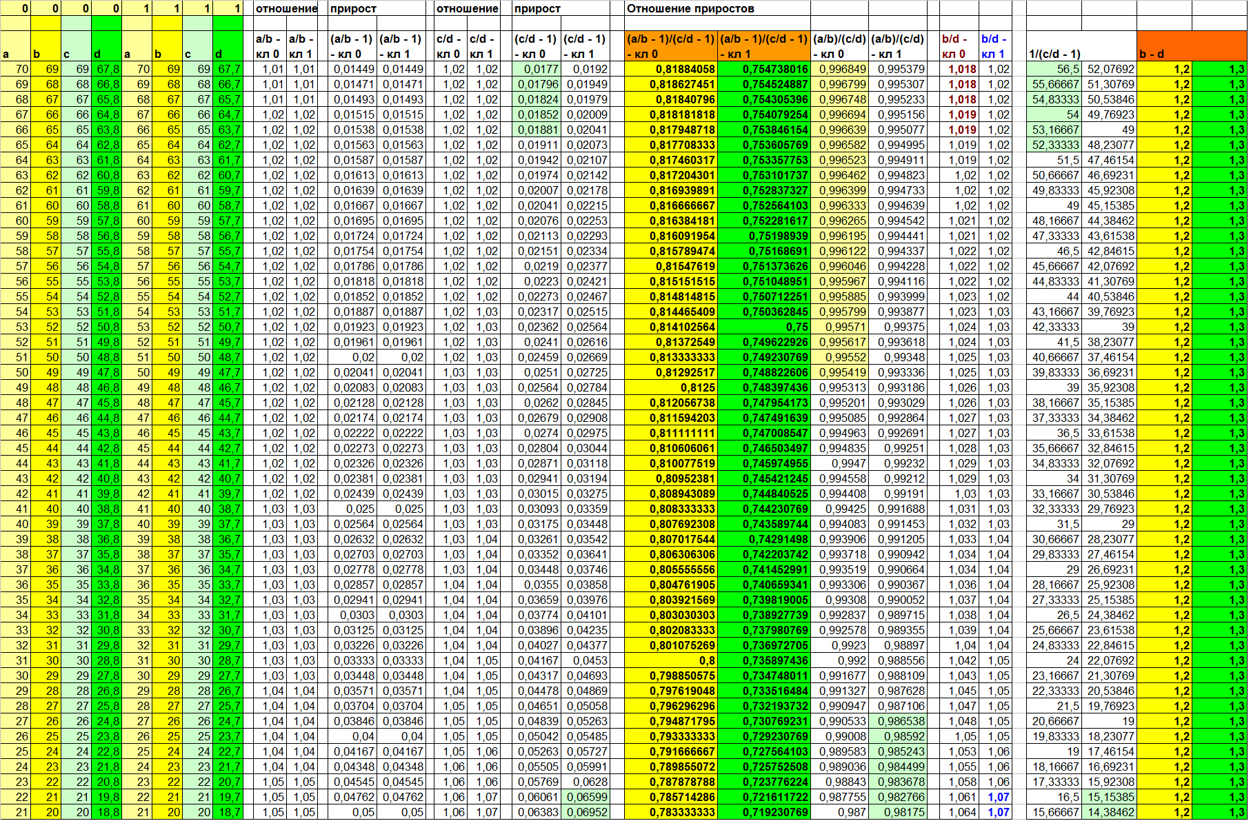
Table 4

The left 8 columns are the actual values ​​of signs a, b, c, d for classes 0 and 1. The values ​​in the remaining columns are calculated in accordance with the function in the header. Values ​​(B - D) in the two right columns.

So, let's see what will give us the use of already known functions, which in Example 1 could make the sample linearly separable.

F(Xi, Xj) = Xi/Xj

As you can see in table 4, the informative relations in this case cannot be found. And even the ratio (B / D) - columns, the values ​​in which we calculated in different ways, does not give us any satisfactory result (the 5th and 6th columns on the right). But what's the matter? We just changed the meaning of the free member only a little! The reason is that in the first example, the free term for different classes had a different sign. And this is exactly what made the sample linearly separable on a sign (B / D).

(A / B) / (C / D) is the ratio of linear bonds or
(A / B - 1) / (C / D - 1) - increment ratio

Let me remind you that in our far-fetched example of the Leprechaun’s computers, such a calculation makes sense: “how much the dependence of performance on turnovers under load changes.”

On our specially fitted and sorted data, we see with the naked eye that the degradation of performance under load on The First machines is slightly higher than on Black Zero machines. (But why, then, do they cost more? Obviously, Black Zero is trying to squeeze out of its nuclear processors more than they can pull, while maintaining reliability. Therefore, they also serve five times less than The First processors! It's unbecoming to sacrifice quality in for marketing, Black Zero!)

Well, let's get back to our relationships. If you look at table 4 again, you will notice one very interesting thing!

The ratio of gains (A / B - 1) / (C / D - 1) makes the sample linearly separable, while the ratio of linear relations (A / B) / (C / D) leaves a rather large range of uncertainty! By the way, here's the answer to the question: "Do both functions always show the same separation capacity?"
(In Table 4, these are columns 7 to 10 on the right. Non-overlapping values ​​are highlighted in color)

Well. It's time to move on to the third example, but for now just remember the following:

• linear relationship and increment ratio functions do not always show the same separation capacity;
• in the example, when the separating ability of the increment ratio function was higher than the separating ability of the linear relationship relation function, the difference function also showed one hundred percent separating ability, but the relationship of pairs of features was not very informative for building an optimal classifier.

The dependence option 3. Xj = K * Xi + C, K! = 1, C = 0

Another special case, but in which, in an unknown relationship, the coefficient, rather than the free term, plays the role.

Let b = a - 1 for both classes, but d = (c * 0.99) for class 0 and (c * 0.98) for class 1)
The results of the calculations are given in Table 5. Let us consider them briefly.


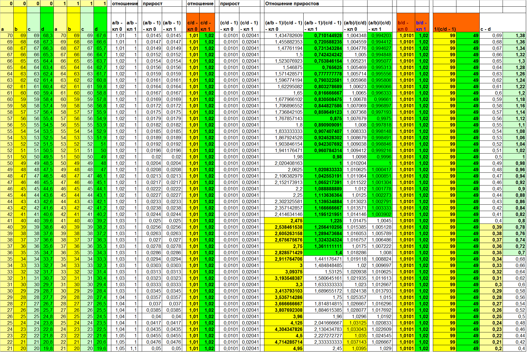
Table 5

Since the contribution to the dependence in this example makes (and only!) The coefficient, the expected function is one hundred percent separability given by the relation function F (Xi, Xj) = Xi / Xj. And the inverse of the increase (3rd and 4th columns on the right) also improves visualization. The ratio of linear dependencies again shows a result that is different from the ratio of increments. And, again, for the worse.

But the function of difference (two right columns), which was stably informative in the previous examples, this time leaves a rather wide zone of uncertainty. And it is noteworthy that it coincides with the zone of uncertainty of the increment ratio function. Compare yourself (columns 1, 2 and 9, 10 on the right; disjoint values ​​of different classes are highlighted in color).

What will the picture be like if the contribution is made by both the coefficient and the free member? Expectedly, none of the relations we considered separately makes the sample linearly separable. However, uncertainty ranges for different calculated columns include different subsets of sample objects! Which of course means that it is most likely possible to build a separating hyperplane on a set of computed attributes, one hundred percent separating objects of different classes.

Let's take an example of the data in Table 6 to consider how this or that function manifested itself at the dependencies that we specified during the formation of these dependencies:

for class 0:

B = A - 1
D = 0,95*B - 0,55

for class 1:

B = A - 1,1
D = 0,965*B - 0,5


Table 6

For the calculated values ​​of the functions of B and D, we see that the simple relation, the ratio of linear connections, the increment and the inverse of the increment gave very similar results. In this case, as we remember, in the past example (table 5) a simple relationship made the sample linearly separable, while the ratio of linear connections left a very wide zone of uncertainty (which, by the way, is due to the excessive use of the function of the relationship of linear relations for the situation in the past) .

We also see that the ratio of increments, in contrast to the previous examples, divided the sample worse than the ratio of linear relations. And the difference function gave even worse results than the ratio of the gains (let me remind you that in all past examples of their effectiveness were the same). It says a lot.

First , the ratio of gains does not necessarily show the same performance as the simple difference.

Secondly , different functions can leave zones of uncertainty of different widths, depending on the true nature of the sought hidden dependence.

Thirdly , depending on the true nature of the desired hidden dependence, different functions can give the best result of the separation of objects of different classes.

Before moving on to what other hidden relationships may exist and how best to organize their search, I will give another example of synthetic data with dependent column D. But this time I will not deliberately give the true function D (a, b, c ). Take a look at table 7 and once again make sure that the three conclusions listed above are correct.


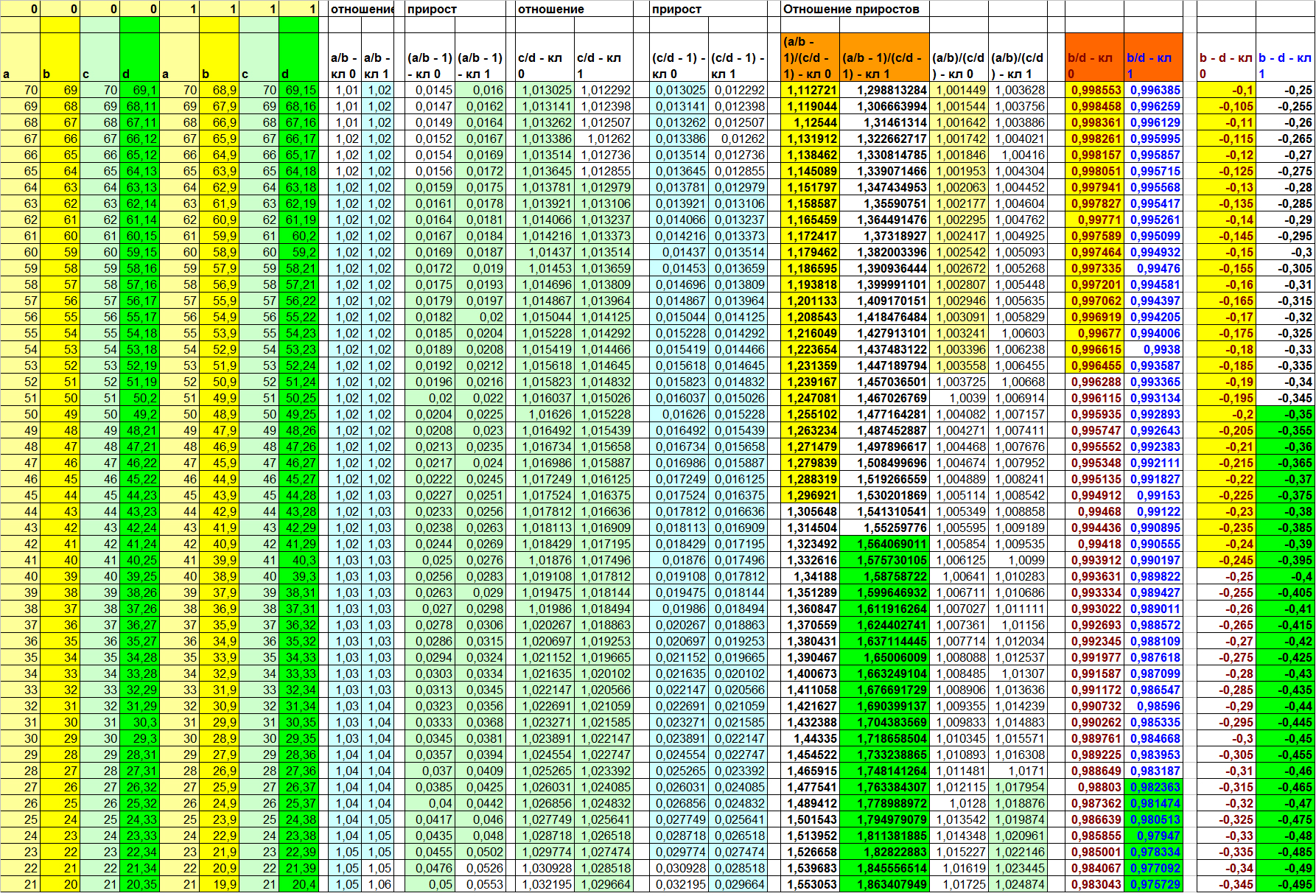
Table 7

What other hidden dependencies might be in the data?

In the examples above, we used a rather primitive linear relationship between features. But can it be that the dependence will be expressed not by a linear function, but by some other, more complex one?

Why not. For example, imagine the data collected by the sensors in the propagation environment of a colony of green microorganisms. If we assume that the concentration of the waste products M is fixed, as well as a number of objective physical parameters of the environment, including the illumination lx, then we can assume that the dependence M (lx) is present. But is such a relationship linear. If we assume that illumination linearly affects the rate of reproduction of bacteria, and the concentration of PZH linearly depends on the number of colonies, then the dependence should be quadratic. The reason is a single-cell breeding method. Namely - cell division. I think that it is unnecessary here to prove that an increase in the rate of single-cell division quadratically (on speed) will affect their numbers in time t. Consequently, we can try, for example, to calculate the ratio (√M / lx), which we consider to be some approximation of the desired linear dependence of the rate of reproduction of green bacteria on the illumination. And if two types of green bacteria really differ in how much light affects their reproduction rate, then this new feature will certainly be able to make its useful contribution to the quality of the final classification algorithm.

Of course, dependencies can be very different, and the basis lies in the meaning embedded in one or another feature. However, let's get away from the semantic load of the signs that describe the objects of the sample, and instead think about how to automate the process of finding hidden dependencies.

Automating the search for dependencies
So, we want to determine if there are hidden dependencies in our attribute description. Let us suppose that we decided not to search for complex algorithms for the selection of signs, and just to test our hypothesis about the existence of a connection for the entire set of attributes N: {X1 ... Xn}. We decide to begin with the pairs of attributes, and for each pair to calculate a certain value — the result of applying for a given pair some function from the set M: {F1 (Xi, Xj) ... Fm (Xi, Xj)}. At the same time, we assume that the set functions have already been selected by us, taking into account some specific features of our task.

It is easy to guess that the number of pairs, for each of which we want to apply m functions from the set M, is the number of combinations of n through 2, that is:

n! / (2! * (n - 2)!) = n * (n - 1) / 2 = (n² - n) / 2 = ½ n² - ½ n

It can be seen that we are dealing with the asymptotic complexity O (n²) .

And from this two conclusions follow:

1. Such a complete search is valid only for a sample with the number of features not exceeding a certain threshold value calculated in advance.
2. Calculation of second-order dependencies, in which columns already calculated on the basis of primary data (as a ratio of increments) are involved, is permissible only if there is a strict algorithm for selecting pairs for such checks. Otherwise, the full pass algorithm will have complexity O (n⁴) . Although in the general case, dependencies of the second order are somehow based, albeit on the sometimes weaker, but still quite informative dependencies of the first order.

Accordingly, it follows from the above that two cases are possible:

1. The number of signs is less than the threshold value, and we can afford to test the hypothesis on each pair.
2. The number of signs exceeds the threshold value, and we need a strategy for selecting couples, on which we will fully test the hypothesis.

Consider first the first case.

The number of signs is less than the threshold value
Strictly speaking, it is not so important for us to identify some kind of dependence in itself, as its different behavior on objects of different classes. Therefore, we can simply omit the moment of checking for dependencies, and instead, immediately check for usefulness of the new column. To do this, it is sufficient to apply one of the known fast classifiers for this column, measuring the average value of the quality metric of interest on the sliding control. And then, if the indicator of the quality metric we are interested in is higher than the threshold value we set, leave the new column, or delete it if the quality has not reached the required one.

Of course, here the thought might come to the reader: what if the new column is calculated based on the original feature, which is already very useful for the final classification algorithm? Indeed, in this case, it turns out that we simply created an extra sign based on what was already available! Pure multicollinearity spawning! So this is what we set the threshold for the classification quality metric for the derived attributes. It is easy to guess that since we are calculating a function from a couple of signs (and not from one!), The result can be just noise, even if both columns were very informative at the input.

It is easy to verify this by the example of synthetic data, where the values ​​in each attribute are independently generated values ​​with the specified mean and deviation. Moreover, so that there is a difference between the means of different classes, and the distribution on the objects of each class is normal (for example, using numpy.random.normal). So, since we a priori generate the values ​​of attributes independently of each other, an attempt to find dependencies only leads to noise, and the derived attributes do not give a satisfactory classification quality.

So, the above example speaks in favor of the fact that if a derived sign turned out to be informative, we can judge that there is a relationship.

The threshold value for derived characteristics can be selected in different ways. Either at once for the entire sample, which is clearly simpler, or individually for each pair. In the second case, we can vary the input threshold value depending on the indicators of the quality metrics of interest on each of the columns submitted to the input.

However, despite the seeming logic of the second choice of the threshold, there is a very unpleasant reef in it. The point is that it is not quite right to choose the value of the quality metric on one of the parent columns as a threshold. The reason is that it may happen that a derived attribute with a slightly lower quality value will indeed be an approximation of a new dependence, and as a result, it may be mistaken on a different set of objects than the parents. This means that its inclusion in the set of features for analysis can radically improve the final quality of the classification!

As for the choice of a common entry threshold for all derived attributes, in my opinion, it is very convenient to choose a threshold based on what values ​​of the quality metric of interest (when used separately!) Have the original columns. So, if for simplicity of example we take Accuracy, then for its values ​​on the original columns [0.52, 0.53, 0.53, 0.54, 0.55, 0.57, 0.59, 0.61, 0.63] the optimal threshold for the derived data will most likely lie somewhere around 0 , 6 (as practice shows). One way or another, this is not so important, because the parameter is trained, and its training will increase the complexity of the algorithm only linearly. When learning this parameter, one way or another, one can build on the Accuracy distribution density of the original features (Accuracy is here only because it has this example!).

In principle, everything is simple. Therefore, we turn to the second case.

The number of signs exceeds the threshold value

This condition means that we cannot afford to carry out a full measurement of the utility for each derivative feature. Or even more: we cannot afford to generate a derivative for each pair of signs. This is understandable: just imagine that we have a thousand signs. In this case, the number of combinations will be equal.

999 * 1000 / 2 = 499 500

And this will be multiplied by the number of functions tested!

And even if our server is able to calculate the quality of the classification by the selected algorithm for a given attribute 100 times per second, to wait almost an hour and a half until the algorithm for generating signs is tested for only one of the functions we have chosen - occupation is at least strange. Although, on the other hand, generating a lot of free time =)

Well, let's get back to our sheep. How can I solve this problem?

Attempting to reduce the number of source characteristics based on their usefulness for classification may not be the best idea, because using the example of synthetic data in the first part of the article, it was clearly shown that a derived characteristic, each of whose parents in its pure form is completely unsuitable for the task of classification, under ideal conditions able to make the sample linearly separable.

How then to be? Apparently, it is necessary to calculate the derived attributes, however, with some limitations.

First, depending on how far the threshold is exceeded in terms of the number of source features, we can only generate part of the original sample objects for evaluating the usefulness of derived features. I will not go into what size of the subsample should be taken - mathematical statistics answers this question quite well.

Secondly, the evaluation of the usefulness of each derived attribute should be carried out on the reduced functionality. Again, depending on the degree of excess of the threshold number of the original. That is, if before that we used to assess the quality of a derived attribute, for example, the method of k nearest neighbors with reduced training functionality, then now we can use it, but with fixed parameters. Or use the method of support vectors with default parameters for weighing the obtained feature set, and then discard columns with a weight below a certain one. Or, for more extreme cases (with the number of initial features), you can simply apply one of the statistical criteria, for example, the simple Rosenbaum Q-test. Unfortunately, the use of such criteria will not help us to select signshaving intermittent peaks in their probability density distributions or simply multidirectional shifted medians.

For example, let the values ​​of the resulting characteristic for classes 1 and -1 be equal respectively: or (for shifted means): It is obvious that in both cases the Rosenbaum criterion considers that the samples do not differ at all. Of course, in this case, the Pearson's criterion will work perfectly, since it involves dividing into a certain number of disjoint intervals and counting the number of values ​​for each interval separately. However, the Pearson criterion will require more time to perform, and this is exactly the parameter that we are trying to optimize in the first - rough approximation. Thirdly, due to the fact that we admit a reduction in the quality of the evaluation of the usefulness of the derived attributes, we also slightly lower the entry threshold.

[9,9,9,9,9,8,8,8,8,8,8,8,8,7,7,7,7,6,6,5,4,3,2,2,1,1,1,1,1,0,0,0,0,0,0,0,0,0]
[9,8,8,7,7,6,6,6,6,6,6,6,6,5,5,5,5,5,5,5,5,5,5,4,4,4,4,4,4,4,3,3,3,3,3,2,2,1,0]



[1,2,2,3,3,3,4,4,4,4,5,5,5,5,5,6,6,6,6] VS [1,1,1,1,2,2,2,2,2,3,3,3,3,4,4,4,5,5,6]





Thus, we get rid of an impressive number of the most uninformative signs with comparatively little blood. But on the remaining ones (again, depending on their number), we can apply methods for a more qualitative assessment of the usefulness of the trait.

To summarize, we are talking about the degradation of the quality of the assessment for the primary rapid rejection of the most non-informative features for the subsequent more qualitative assessment of the remaining ones.

Well, it's time, perhaps, to complete. Briefly summarize all the above, it is worth noting the following points.

findings

• It is often possible to find hidden dependencies F (Xi, Xj), which are able to act as independent features and improve the quality of classification, for a characteristic description of data in classification problems.
• , .
• , .
• k*(n² — n) / 2, k — , n — .
• .
• If the number of initial signs exceeds a certain threshold value, the verification of derived attributes should be carried out in two stages: rapid rejection of the most non-informative derivative features and the subsequent more qualitative analysis of the remaining ones. Hypothetically, it is possible to calculate the derived attributes F (Xi, Xj) of the set of features M ', which will give us the application of the principal component method to the original set of features M, but the question arises whether all hidden dependencies can be manifested in this case.

Well, that's all for this time. And yes, now we can definitely help the leprechauns more effectively find dissidents among their relatives!