Non-standard clustering 4: Self-Organizing Maps, subtleties, improvements, comparison with t-SNE
Part One - Affinity Propagation
Part Two - DBSCAN
Part Three - Time Series Clustering
Part Four - Self-Organizing Maps (SOM)
Part Five - Growing Neural Gas (GNG)
Self-organizing maps (SOM, Kohonen self-organizing maps) is a familiar classical construction. They are often commemorated in machine-learning courses under the sauce, “and yet neural networks can do this.” SOM managed to survive the take-off in 1990-2000: then they were predicted a great future and created new and new modifications. However, in the 21st century, SOM is gradually receding into the background. Although new developments in the field of self-organizing maps are still underway (mostly in Finland, the birthplace of Kohonen), even in the native field of visualization and clustering of the Kohonen map data is increasingly inferior to t-SNE.
Let's try to understand the intricacies of SOMs, and find out if they were deservedly forgotten.
')

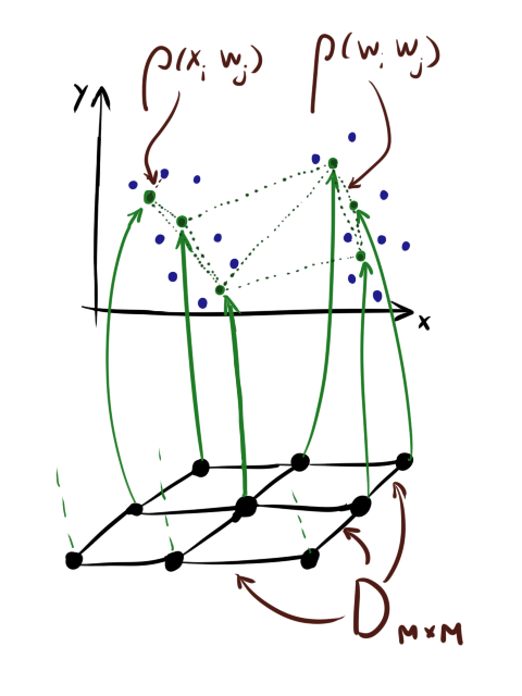
In brief, let me remind you the standard learning algorithm SOM [1]. Hereinafter X ( d timesN ) - matrix with input data, where N - the number of elements in the data set, and d - the dimension of the data. W - matrix of scales ( d timesM ) where M - the number of neurons in the map. eta - learning speed sigma - coefficient of cooperation (see below), E - the number of epochs.
D ( M timesM ) - matrix of distances between neurons in the layer. I draw your attention that the last matrix is not the same as left | vecwi− vecwj right | . For neurons there are two distances : the distance in the layer ( D ) and the difference between the values.
Also note that although neurons are often drawn for convenience as if they were “strung” on a square grid, this does not mean that they are stored as a tensor. sqrtM times sqrtM timesd . Mesh personifies D .
We introduce immediately gamma and alpha - indicators of the attenuation of the learning rate and the attenuation of cooperation, respectively. Although strictly speaking they are not mandatory, without them it is almost impossible to come together to a decent result.
Algorithm 1 (standard SOM learning algorithm):
Entrance: X , eta , sigma , gamma , alpha , E
Each era of learning, we iterate over the elements of the input dataset. For each item we find the one closest to it. x neuron, then we update its weight and the weight of all its neighbors according to the layer depending on the distance to x and the coefficient of cooperation sigma . The more sigma , the more neurons effectively update the weights at each step. The picture below is a graphic interpretation of steps A1.2.2.1-A1.2.2.4 for the case when sigma large (1) and when small (2) with the same learning speed and the nearest vector.
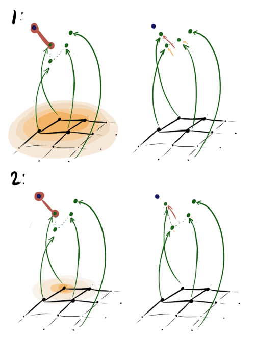
In the first case hij close to one and to vecx not only the nearest vector moves, but also its first neighbor and even, slightly less, the second neighbor. In the second case, the same neighbors move quite a bit. Note that in both cases the fourth vector with the same left | vecwi− vecwj right | from the nearest vector, but with a much larger Dij does not move.
Several epochs of learning Kohonen maps for clarity:

If my brief reminder algorithm was not enough, read this article, where the steps in A1 are discussed in more detail.
Thus, the main ideas of SOM:
Immediately suggests several trivial modifications:
A slightly less obvious modification of self-organizing cards, in which their strength and uniqueness consist, but which is constantly forgotten, lies in the initialization stage W and D . In the examples, the Kohonen layer is constantly depicted as a grid, but this is by no means necessary. On the contrary, it is strongly advised to adjust the relative position of the neurons ( D ) in the data layer.
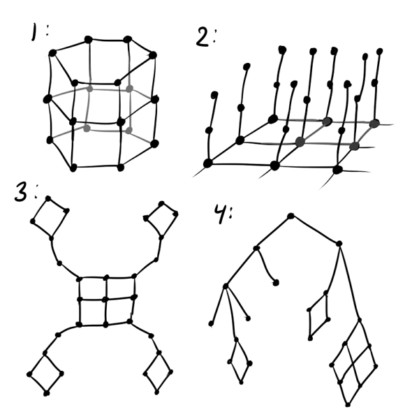
At a minimum, instead of a regular grid, it is better to use a hexagonal one: a square grid distorts the results in favor of straight lines, and it is less pleasant to look at than a hexagonal one. If it is assumed that the data is cyclic, it is worth initializing D as if neurons are on a tape or even on a torus (see figure below, number 1). If you are trying to fit three-dimensional data in the SOM that does not necessarily fall on the hyperfolding, you should use the “fleecy carpet” structure (2). If it is known that some clusters can defend far from others, try the “petal” layer structure (3). It’s very good if the data is known to have a certain hierarchy: then it’s possible to D You can take the distance matrix of the graph of this hierarchy (4).
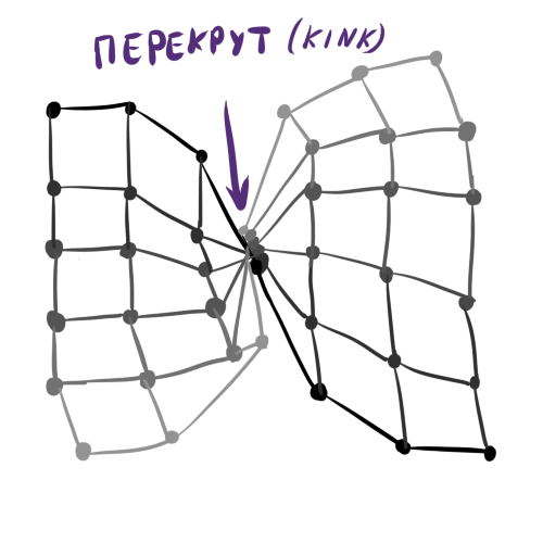
Generally, D limited to your imagination, knowledge of the data and convenience of the subsequent visualization of neurons. Because of the latter factor, it is not worth doing, for example, the Kohonen cubic layer. Establishing your own order between neurons is a powerful tool, but remember that the more complex the structure D the harder it is to initialize initial weights in W and the more likely it is to get the so-called torsion (kink) in the Kohonen layer at the output. Torsion is a learning defect when W globally match D and the data, with the exception of some special points in which the layer is twisted, stretches unnaturally or is divided between two clusters. In this case, the SOM learning algorithm cannot get out of this state without destroying an already established structure. It is easy to see that torsion is an analogue of a deep local minimum in the training of ordinary neural networks.
An abstract example of the classic torsion:
An example of a twist on synthetic data when trying to fit a long curve into clusters. The upper left and right petals look believable, but the allocated space spoils the order.

By initializing the weights in the layer at random, you practically guarantee yourself a bad result at the output. Must be constructed W so that in each specific area the density of neurons approximately corresponds to the density of the data. Alas, without extrasensory abilities or additional information about dataset, this is quite difficult to do.
Therefore, it is often necessary to do so that the neurons are simply uniformly scattered throughout the data space without intersections (as in the figure in the middle), and put up with the fact that not in all areas the density of neurons will correspond to data density.
This idea was originally proposed by Kohonen [1], and then summarized by his followers [4]. What if you take away or add to the update of the neuron, the winner of the update of its neighbors? Mathematically, it looks like this: Step A1.2.2.4 for the winner's neuron is replaced by
Where lambda - Relaxation option. Updates of the remaining neurons remain unchanged or a part of the relaxing term is added to them. Sounds weird; it turns out that if lambda<0 and the neuron has many neighbors, it can even roll back from vecx ? If you do not use the top limit on the length of the vector, it is:
With a negative lambda a neuron seems to be pulling its neighbors to itself, and if positive, it tends to jump out of their surroundings. The difference is especially noticeable at the beginning of training. Here is an example of the SOM state after the first epoch for the same initial configuration and negative, zero and positive lambda respectively:
Due to the effects described above lambda<0 neurons scatter more broadly when lambda>0 - drawn out. Accordingly, in the first case, the coating will be more uniform, and in the second, small isolated clusters and outliers will have a greater effect. In the latter case, a possible torsion is also visible at the top of the graph. The literature advises lambda in[−1;1] , but I found that good results can be obtained even with much larger in modulus values. Please note that the added item includes hij which in turn depends on sigma . Consequently, the above-described technique will play a large role at the beginning of training - at the stage of cooperation.
It often happens that after the main loop of the algorithm it turns out that even though the SOM neurons cling to something, their density on the clusters is quite comparable with the density in places where there are no clusters. Analyzing in such conditions is quite difficult. Narni Manukyan and the team propose [5] a rather simple solution: after the main algorithm, run another neuron fitting cycle.
Algorithm 2, Cluster refinement phase (cluster adjustment phase):
Entrance: X , etaCR , sigmaCR , gammaCR , alphaCR , ECR
Although the algorithm looks and is very similar to A1, note that now we are not looking for the nearest neuron, but simply push all neurons to x . Due to interaction vecx− vecwj in the exponent in A2.2.2.2 and at the stage of updating the weights only the neurons that are in a certain ring from vecx . For clarity, look at the five epochs of adjustment:
More accurately: the more fine tuning is in the CR phase, the better the clusters are visible, but the more local information about the cluster shape is lost. After several epochs, only data on the elongation of clots remains. CR can collapse several folds located nearby, and when too large sigmaCR , you risk just spoiling the structure obtained in the main step, as in the picture below:
However, the last problem can be avoided if we take some function instead of an exponent, which after some maximum value turns to 0.
The authors of the article advise to use the same instead of a separate parameter of learning speed. sigmaCR but it frankly doesn't work: if sigmaCR large (of the order of unity), the algorithm goes hand in hand, if small (0.01), then nothing is updated at all. Strange, perhaps, they had some good data or a fitted vector of importance of variables?
So far, I have not said a word about data clustering using SOM. Built with D and W the grid is a fun visualization, but by itself it says nothing about the number of clusters. Moreover, I would even say that beautiful multicolored grids that you can google at the request of “SOM visualization” are more likely a reception for press releases and popular articles than a really useful thing.
The easiest way to determine the number of data bunches in a crease is to look thoughtfully at a so-called U-matrix . This is a kind of visualization of Kohonen maps, where the distance between them is shown along with the values of the neurons. This way you can easily determine where the clusters are in contact, and where the border lies.
A more interesting way is to run over the resulting matrix. W some other clustering algorithm. For example, DBSCAN is suitable , especially with the CR modification of the SOM described above. The distance function of the second algorithm should be combined from the distance along the grid in the layer ( D ) and the real distance between neurons ( left | vecwi− vecwj right | ) so as not to lose topological information about the crease.
But more advanced seems to be the accumulation of relevant information about clusters right while the main algorithm is running. Ehren Golge and Pinar Daigulu suggest [6] to remember every epoch of the basic algorithm operation how many times the neuron was activated (i.e., the neuron turned out to be the winner or its weight was updated, because the neuron closest in layer was the winner), and , whether the neuron person represents a cluster or hangs in empty space.
Algorithm 3, Rectifying SOM (A1 with changes):
Entrance: X , eta , sigma , gamma , alpha , E
The more often the neuron is the winner, the greater the likelihood that it is somewhere in the thick of the cluster, and not outside it. Note that the total count of neurons accumulates with a multiplier. 1/ eta : the lower the learning speed, the more weight WC will have. This is done so that the last epochs of the cycle contribute more than the first. This can be done in other ways, so slightly attach to this particular form.
ES is a dimensionless quantity, its absolute values do not have a special meaning. Simply, the greater the value, the greater the chance that the neuron clings to something meaningful. After the end of A3, the resulting vector should be somehow normalized. After applying ES to the neurons, you will get something like this:
Large red dots represent neurons with a high score of arousal, small red-violet ones with a small one. Please note that the RSOM is sensitive to the method of final processing of ES and to clusters of different density in the data (see the lower right corner of the picture). Make sure that you specify more epochs than is necessary for the convergence of the algorithm, so that ES accurately has time to accumulate the correct values.
It is best, of course, to use both the RSOM and the additional clustering atop and viewing the visualization with the eyes.
The review did not enter
It would seem that SOM wins in computational complexity, but you shouldn’t rejoice ahead of time without seeing N 2 under the O-large.M depends on the desired resolution of the self-organizing map, which depends on the spread and heterogeneity of the data, which, in turn, implicitly depends onN and d . So in real life, complexity is something like O ( d N 32 E) .
The following table shows the strengths and weaknesses of the SOM and t-SNE. It is easy to understand why self-organizing maps have given way to other clustering methods: although visualization with Kohonen maps is more meaningful, it allows the growth of new neurons and setting the desired topology on neurons, the degradation of the algorithm with larged strongly undermines the demand for SOM in modern data science. In addition, if visualization using t-SNE can be used immediately, self-organizing maps need post-processing and / or additional visualization efforts. An additional negative factor - problems with initializationW and torsion. Does this mean that self-organizing maps are a thing of the past data science?
Not really.No, no, yes, and sometimes it is necessary to process not very multidimensional data - for this it is possible to use SOM. The visualizations are really pretty and spectacular. If you do not be lazy to apply the refinement of the algorithm, SOM perfectly finds clusters on hyperlinks.
Thanks for attention.I hope my article will inspire someone to create new SOM-visualizations. From github you can download the code with a minimal example of SOM with the main optimizations proposed in the article and look at the animated map training. Next time I will try to consider the “neural gas” algorithm, which is also based on competitive learning.
[1]: Self-Organizing Maps, book; Teuvo Kohonen
[2]: Energy functions for self-organizing maps; Tom Heskesa, Theoretical Foundation SNN, University of Nijmegen
[3]: bair.berkeley.edu/blog/2017/08/31/saddle-efficiency
[4]: Winner-Relaxing Self-Organizing Maps, Jens Christian Claussen
[5]: Data-Driven Cluster Reinforcement and Sparsely-Matched Self-Organizing Maps; Narine Manukyan, Margaret J. Eppstein, and Donna M. Rizzo
[6]: Recording text from Web Images; Eren Golge & Pinar Duygulu
[7]: An Alternative Approach for Binary and Categorical Self-Organizing Maps; Alessandra Santana, Alessandra Morais, Marcos G. Quiles
[8]: Temporally Asymmetric Learning Multi-Winner Self-Organizing Maps
[9]: Magnification Control in Self-Organizing Maps and Neural Gas; Thomas Villmann, Jens Christian Claussen
[10]: Embedded Selection for Self-Organizing Maps; Ryotaro Kamimural, Taeko Kamimura
[11]: Initialization Issues in Self-organizing Maps; Iren Valova, George Georgiev, Natacha Gueorguieva, Jacob Olsona
[12]: Self-organizing Map Initialization; Mohammed Attik, Laurent Bougrain, Frederic Alexandre
Part Two - DBSCAN
Part Three - Time Series Clustering
Part Four - Self-Organizing Maps (SOM)
Part Five - Growing Neural Gas (GNG)
Self-organizing maps (SOM, Kohonen self-organizing maps) is a familiar classical construction. They are often commemorated in machine-learning courses under the sauce, “and yet neural networks can do this.” SOM managed to survive the take-off in 1990-2000: then they were predicted a great future and created new and new modifications. However, in the 21st century, SOM is gradually receding into the background. Although new developments in the field of self-organizing maps are still underway (mostly in Finland, the birthplace of Kohonen), even in the native field of visualization and clustering of the Kohonen map data is increasingly inferior to t-SNE.
Let's try to understand the intricacies of SOMs, and find out if they were deservedly forgotten.
')
The basic ideas of the algorithm
In brief, let me remind you the standard learning algorithm SOM [1]. Hereinafter X ( d timesN ) - matrix with input data, where N - the number of elements in the data set, and d - the dimension of the data. W - matrix of scales ( d timesM ) where M - the number of neurons in the map. eta - learning speed sigma - coefficient of cooperation (see below), E - the number of epochs.
D ( M timesM ) - matrix of distances between neurons in the layer. I draw your attention that the last matrix is not the same as left | vecwi− vecwj right | . For neurons there are two distances : the distance in the layer ( D ) and the difference between the values.
Also note that although neurons are often drawn for convenience as if they were “strung” on a square grid, this does not mean that they are stored as a tensor. sqrtM times sqrtM timesd . Mesh personifies D .
We introduce immediately gamma and alpha - indicators of the attenuation of the learning rate and the attenuation of cooperation, respectively. Although strictly speaking they are not mandatory, without them it is almost impossible to come together to a decent result.
Algorithm 1 (standard SOM learning algorithm):
Entrance: X , eta , sigma , gamma , alpha , E
- Initialize W
- E time:
- Shuffle index list randomly order: = shuffle ( [0,1, dots,N−2,N−1] )
- For each idx from order:
- vecx:=X[idx] // Take a random vector from X
- i:= arg minj left | vecx− vecwj right | // Find the number of the neuron nearest to it
- forallj:hij:=eDij/ sigma2 // Find the coefficient of proximity of neurons on the grid. Notice that hii always 1
- forallj: vecwj:= vecwj+ etahij( vecx− vecwj)
- eta : = gamma eta
- sigma : = alpha sigma
Each era of learning, we iterate over the elements of the input dataset. For each item we find the one closest to it. x neuron, then we update its weight and the weight of all its neighbors according to the layer depending on the distance to x and the coefficient of cooperation sigma . The more sigma , the more neurons effectively update the weights at each step. The picture below is a graphic interpretation of steps A1.2.2.1-A1.2.2.4 for the case when sigma large (1) and when small (2) with the same learning speed and the nearest vector.
In the first case hij close to one and to vecx not only the nearest vector moves, but also its first neighbor and even, slightly less, the second neighbor. In the second case, the same neighbors move quite a bit. Note that in both cases the fourth vector with the same left | vecwi− vecwj right | from the nearest vector, but with a much larger Dij does not move.
Several epochs of learning Kohonen maps for clarity:
If my brief reminder algorithm was not enough, read this article, where the steps in A1 are discussed in more detail.
Thus, the main ideas of SOM:
- Forcing the introduction of some order between neurons. D gently transferred to W into the data space.
- Winner Takes All (WTA) Strategy. At each step of the training, we determine the closest “winning” neuron and, based on this knowledge, weights are updated.
- Cooperation turns into egoism rightarrow global approximate adjustment develops into an exact local. Until sigma big, the noticeable part is updated W and the WTA strategy is not so visible when sigma tends to zero w updated one by one.
Immediately suggests several trivial modifications:
- It is not necessary to use a Gaussian to calculate hij in step A1.2.2.3. The first candidate for alternatives is the Cauchy distribution. As you know, it has heavier tails: more neurons will change at the stage of cooperation.
- Damping eta and sigma do not have to be exponential. The attenuation curve in the form of a sigmoid or a Gaussian branch can give the algorithm more time for a coarse adjustment.
- It is not necessary to spin in a loop exactly E time. You can stop the iteration if the values of W will not change over several epochs.
- Training resembles the usual SGD. "Reminds", because there is no energy function that this process would optimize [2]. Strict math spoils us step A1.2.2.1 - taking the nearest vector. There are modifications SOM, where the energy is still there, but we already go into the details. The point is that it does not interfere with using at step A1.2.2.4 instead of the usual updates of the weights, say, Nesterov's momentum (Nesterov momentum).
- Adding small random perturbations to the gradient, although of less benefit than in the case of ordinary multilayer neural networks, still looks like a useful technique for avoiding saddle points [3].
- Self-organizing maps support learning by subsamples (batches) [1]. Their use allows you to train faster and smoother skip bad configurations. W
- Do not forget about the normalization of input values and the use of the weights vector of input variables, if you know that some features are more important than others.
Neuron topology
A slightly less obvious modification of self-organizing cards, in which their strength and uniqueness consist, but which is constantly forgotten, lies in the initialization stage W and D . In the examples, the Kohonen layer is constantly depicted as a grid, but this is by no means necessary. On the contrary, it is strongly advised to adjust the relative position of the neurons ( D ) in the data layer.
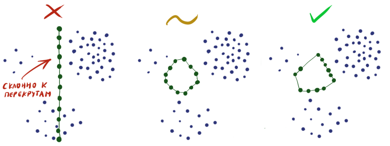
At a minimum, instead of a regular grid, it is better to use a hexagonal one: a square grid distorts the results in favor of straight lines, and it is less pleasant to look at than a hexagonal one. If it is assumed that the data is cyclic, it is worth initializing D as if neurons are on a tape or even on a torus (see figure below, number 1). If you are trying to fit three-dimensional data in the SOM that does not necessarily fall on the hyperfolding, you should use the “fleecy carpet” structure (2). If it is known that some clusters can defend far from others, try the “petal” layer structure (3). It’s very good if the data is known to have a certain hierarchy: then it’s possible to D You can take the distance matrix of the graph of this hierarchy (4).
Generally, D limited to your imagination, knowledge of the data and convenience of the subsequent visualization of neurons. Because of the latter factor, it is not worth doing, for example, the Kohonen cubic layer. Establishing your own order between neurons is a powerful tool, but remember that the more complex the structure D the harder it is to initialize initial weights in W and the more likely it is to get the so-called torsion (kink) in the Kohonen layer at the output. Torsion is a learning defect when W globally match D and the data, with the exception of some special points in which the layer is twisted, stretches unnaturally or is divided between two clusters. In this case, the SOM learning algorithm cannot get out of this state without destroying an already established structure. It is easy to see that torsion is an analogue of a deep local minimum in the training of ordinary neural networks.
An abstract example of the classic torsion:
An example of a twist on synthetic data when trying to fit a long curve into clusters. The upper left and right petals look believable, but the allocated space spoils the order.
By initializing the weights in the layer at random, you practically guarantee yourself a bad result at the output. Must be constructed W so that in each specific area the density of neurons approximately corresponds to the density of the data. Alas, without extrasensory abilities or additional information about dataset, this is quite difficult to do.
Therefore, it is often necessary to do so that the neurons are simply uniformly scattered throughout the data space without intersections (as in the figure in the middle), and put up with the fact that not in all areas the density of neurons will correspond to data density.
Winner relaxation / winner enhancing
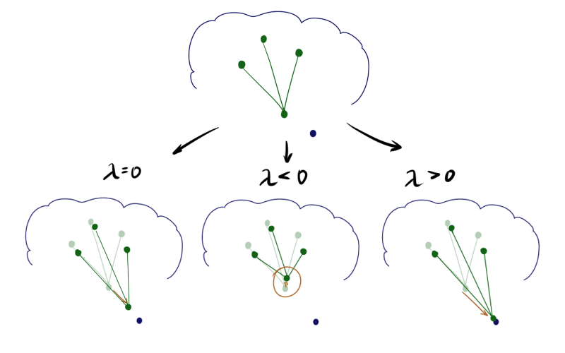
This idea was originally proposed by Kohonen [1], and then summarized by his followers [4]. What if you take away or add to the update of the neuron, the winner of the update of its neighbors? Mathematically, it looks like this: Step A1.2.2.4 for the winner's neuron is replaced by
vecwi:= vecwi+ eta(( vecx− vecwi)+ lambda sumj neqihij( vecx− vecwj))
Where lambda - Relaxation option. Updates of the remaining neurons remain unchanged or a part of the relaxing term is added to them. Sounds weird; it turns out that if lambda<0 and the neuron has many neighbors, it can even roll back from vecx ? If you do not use the top limit on the length of the vector, it is:
With a negative lambda a neuron seems to be pulling its neighbors to itself, and if positive, it tends to jump out of their surroundings. The difference is especially noticeable at the beginning of training. Here is an example of the SOM state after the first epoch for the same initial configuration and negative, zero and positive lambda respectively:
Due to the effects described above lambda<0 neurons scatter more broadly when lambda>0 - drawn out. Accordingly, in the first case, the coating will be more uniform, and in the second, small isolated clusters and outliers will have a greater effect. In the latter case, a possible torsion is also visible at the top of the graph. The literature advises lambda in[−1;1] , but I found that good results can be obtained even with much larger in modulus values. Please note that the added item includes hij which in turn depends on sigma . Consequently, the above-described technique will play a large role at the beginning of training - at the stage of cooperation.
Cluster refinement phase
It often happens that after the main loop of the algorithm it turns out that even though the SOM neurons cling to something, their density on the clusters is quite comparable with the density in places where there are no clusters. Analyzing in such conditions is quite difficult. Narni Manukyan and the team propose [5] a rather simple solution: after the main algorithm, run another neuron fitting cycle.
Algorithm 2, Cluster refinement phase (cluster adjustment phase):
Entrance: X , etaCR , sigmaCR , gammaCR , alphaCR , ECR
- ECR time:
- Shuffle index list randomly order: = shuffle ( [0,1, dots,N−2,N−1] )
- For each idx from order:
- vecx:=X[idx] // Take a random vector from X
- forallj:hij:=e left | vecx− vecwj right |/ sigma2CR // Find the coefficient of proximity of neurons to the selected data element
- forallj: vecwj:= vecwj+ etaCRhij( vecx− vecwj)
- etaCR : = gammaCR etaCR
- sigmaCR : = alphaCR sigmaCR
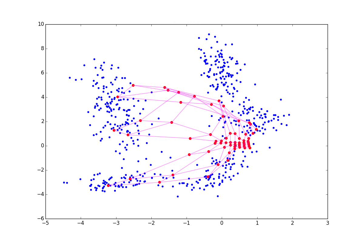
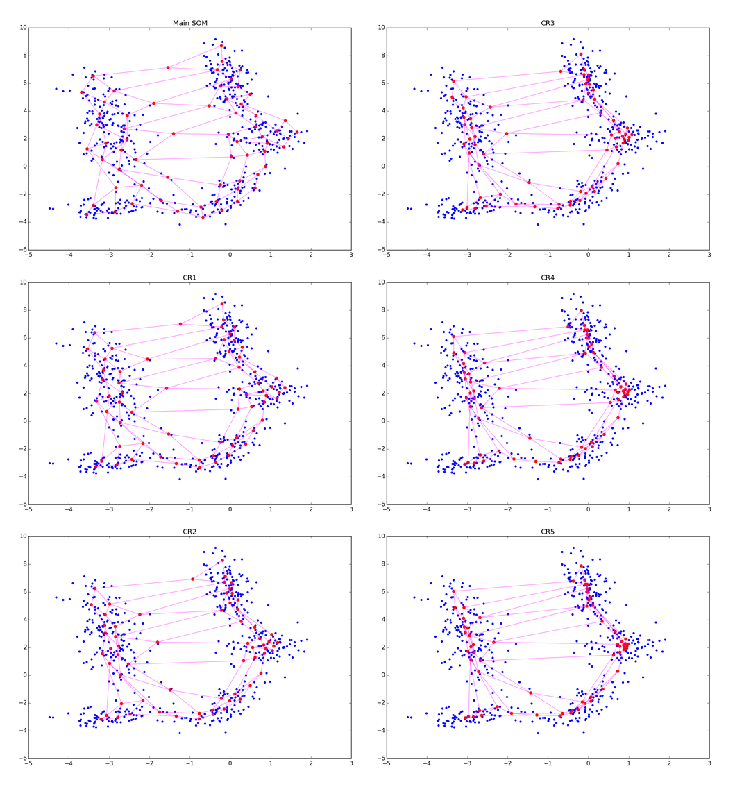
Although the algorithm looks and is very similar to A1, note that now we are not looking for the nearest neuron, but simply push all neurons to x . Due to interaction vecx− vecwj in the exponent in A2.2.2.2 and at the stage of updating the weights only the neurons that are in a certain ring from vecx . For clarity, look at the five epochs of adjustment:
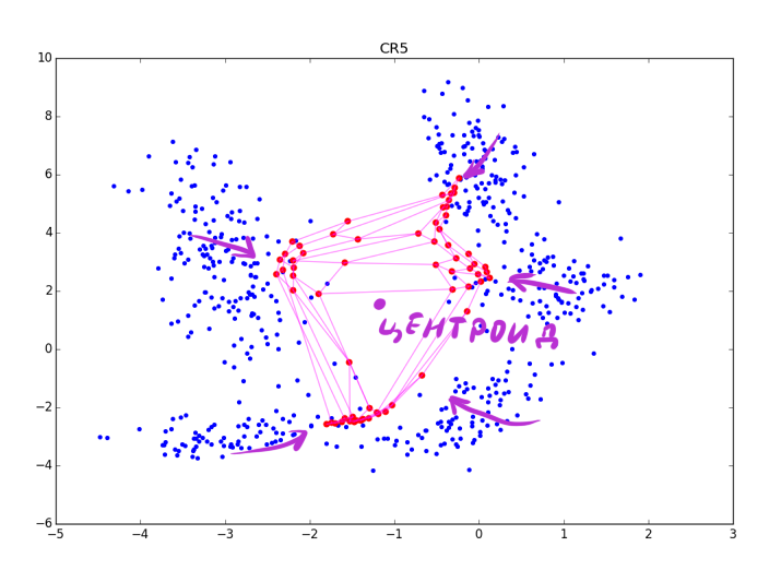
More accurately: the more fine tuning is in the CR phase, the better the clusters are visible, but the more local information about the cluster shape is lost. After several epochs, only data on the elongation of clots remains. CR can collapse several folds located nearby, and when too large sigmaCR , you risk just spoiling the structure obtained in the main step, as in the picture below:
However, the last problem can be avoided if we take some function instead of an exponent, which after some maximum value turns to 0.
The authors of the article advise to use the same instead of a separate parameter of learning speed. sigmaCR but it frankly doesn't work: if sigmaCR large (of the order of unity), the algorithm goes hand in hand, if small (0.01), then nothing is updated at all. Strange, perhaps, they had some good data or a fitted vector of importance of variables?
Visualization, Rectifying SOM
So far, I have not said a word about data clustering using SOM. Built with D and W the grid is a fun visualization, but by itself it says nothing about the number of clusters. Moreover, I would even say that beautiful multicolored grids that you can google at the request of “SOM visualization” are more likely a reception for press releases and popular articles than a really useful thing.
The easiest way to determine the number of data bunches in a crease is to look thoughtfully at a so-called U-matrix . This is a kind of visualization of Kohonen maps, where the distance between them is shown along with the values of the neurons. This way you can easily determine where the clusters are in contact, and where the border lies.
A more interesting way is to run over the resulting matrix. W some other clustering algorithm. For example, DBSCAN is suitable , especially with the CR modification of the SOM described above. The distance function of the second algorithm should be combined from the distance along the grid in the layer ( D ) and the real distance between neurons ( left | vecwi− vecwj right | ) so as not to lose topological information about the crease.
But more advanced seems to be the accumulation of relevant information about clusters right while the main algorithm is running. Ehren Golge and Pinar Daigulu suggest [6] to remember every epoch of the basic algorithm operation how many times the neuron was activated (i.e., the neuron turned out to be the winner or its weight was updated, because the neuron closest in layer was the winner), and , whether the neuron person represents a cluster or hangs in empty space.
Algorithm 3, Rectifying SOM (A1 with changes):
Entrance: X , eta , sigma , gamma , alpha , E
- Initialize W
- Initialize Es= vec0 // Excitement score - full account of neuron excitation
- E time:
- Initialize WC= vec0 // Win count - the account of the excitation of the neuron in the current era
- Shuffle index list randomly order: = shuffle ( [0,1, dots,N−2,N−1] )
- For each idx from order:
- vecx:=X[idx] // Take a random vector from X
- i:= arg minj left | vecx− vecwj right | // Find the number of the neuron nearest to it
- forallj:hij:=eDij/ sigma2 // Find the coefficient of proximity of neurons on the grid. Notice that hii always 1
- forallj: vecwj:= vecwj+ etahij( vecx− vecwj)
- forallj:WCj:=WCj+hij // Update the current activation account
- eta : = gamma eta
- sigma : = alpha sigma
- forallj:ES:=ES+WC/ eta // Accumulate the total score
The more often the neuron is the winner, the greater the likelihood that it is somewhere in the thick of the cluster, and not outside it. Note that the total count of neurons accumulates with a multiplier. 1/ eta : the lower the learning speed, the more weight WC will have. This is done so that the last epochs of the cycle contribute more than the first. This can be done in other ways, so slightly attach to this particular form.
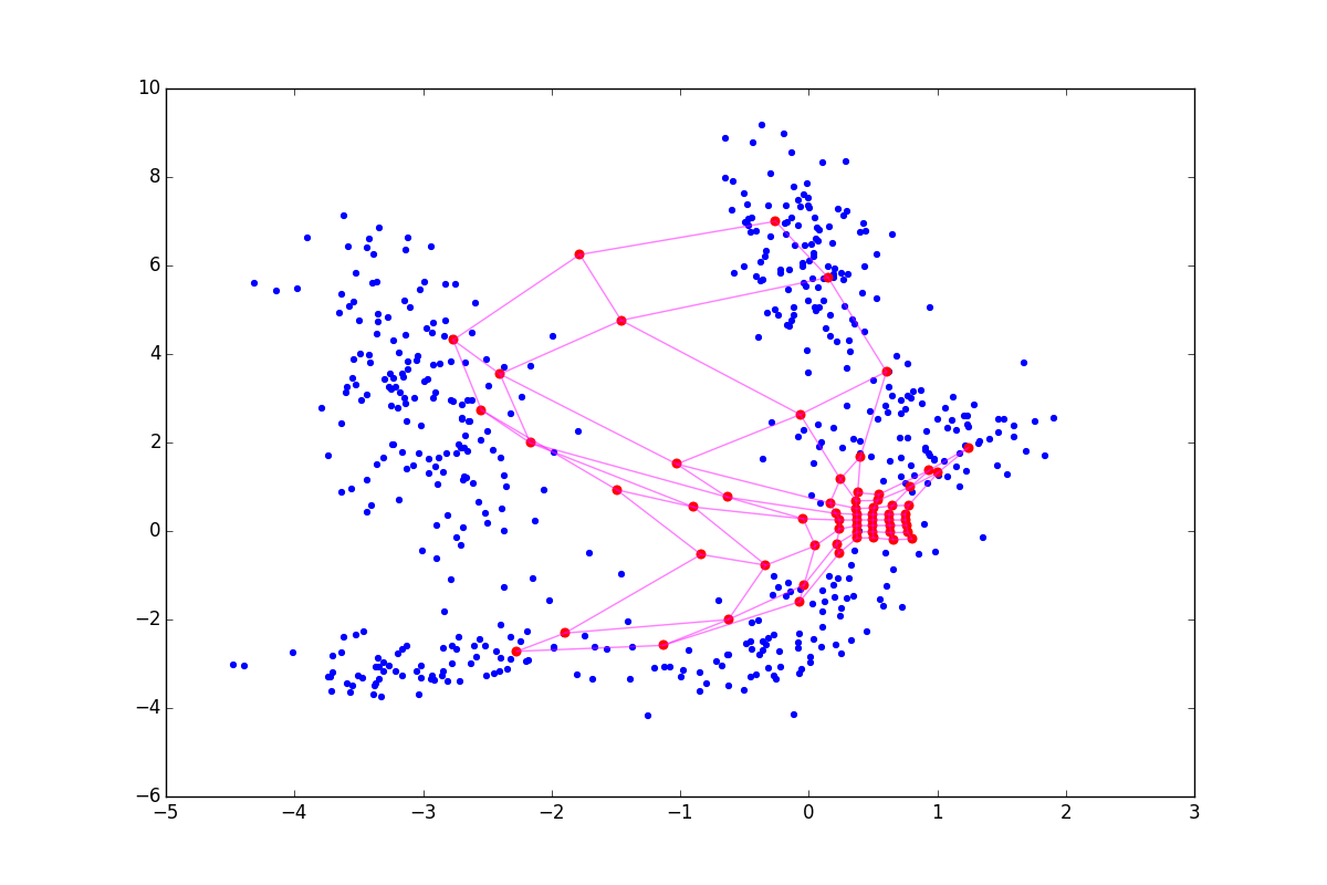
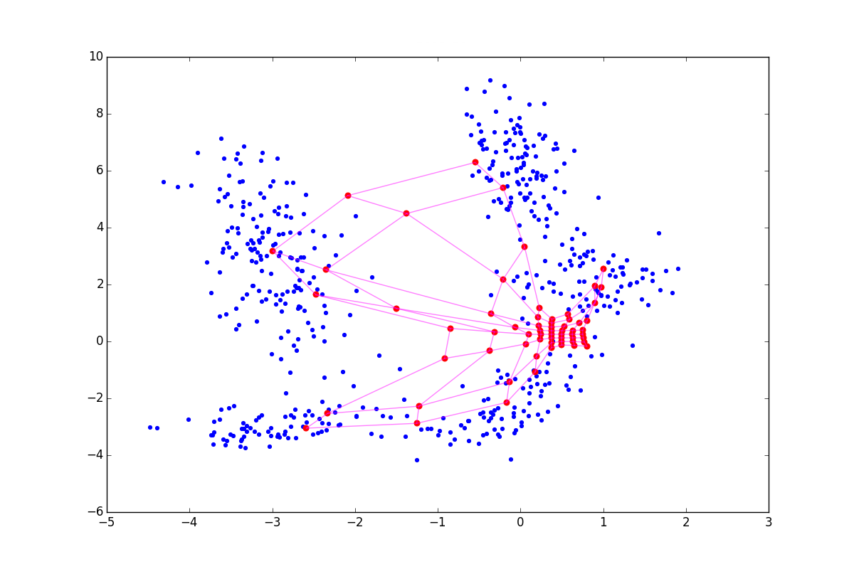
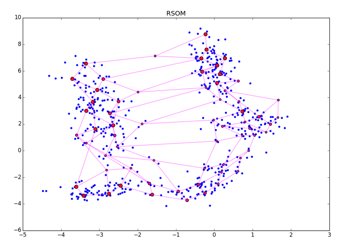
ES is a dimensionless quantity, its absolute values do not have a special meaning. Simply, the greater the value, the greater the chance that the neuron clings to something meaningful. After the end of A3, the resulting vector should be somehow normalized. After applying ES to the neurons, you will get something like this:
Large red dots represent neurons with a high score of arousal, small red-violet ones with a small one. Please note that the RSOM is sensitive to the method of final processing of ES and to clusters of different density in the data (see the lower right corner of the picture). Make sure that you specify more epochs than is necessary for the convergence of the algorithm, so that ES accurately has time to accumulate the correct values.
It is best, of course, to use both the RSOM and the additional clustering atop and viewing the visualization with the eyes.
Other
The review did not enter
- Modifications of SOM for working with categorical data [7], sequences, pictures, and other types of data that are non-native to SOM, [1].
- Work related to the time asymmetry of the proximity functions of neurons on the grid.
The author argues that it allows you to deal with torsion [8]. - Studies related to control over the extent of data coverage by neurons (fight against distortions at the edges of the dataset) [9].
- The accumulation of information about the importance of certain inputs [10].
- Data coding using SOM [1].
- Clever ways to initialize W [11] [12].
- Ability to add an additional component of elasticity . Elasticity is an analogue of regularization in ordinary neural networks, prohibiting configurations that are too complicated.
- Emission detection. A rather simple idea: after a certain epoch, when the map has already more or less converged, you can begin to check whether the distance from x to the nearest neuron. If for several epochs the distance is greater than the specified parameter and does not change, you can mark the sample data as an outlier (and alternatively, even exclude from the update step). Minus: detects outliers only “outside” dataset, but not in its thickness.
- Many other interesting, but too special things.
Comparison of SOM and t-SNE
| SOM | t-SNE | |
|---|---|---|
| Complexity | O(dENM) | Barnes-Hut t-SNE with kNN optimization - O(dEN logN) , but other implementations may be more computationally intensive, right up to O ( d E N 2 ) |
| The number of hyperparameters | 3-5, perhaps much more + distance matrix on neurons. Mandatory number of epochs, learning rate and the initial rate of cooperation. Also, the attenuation of the learning rate and the coefficient of cooperation are often indicated, but they almost never cause problems. | 3-4, maybe more + metrics on data. Mandatory number of epochs, learning rate and perplexity, often occurs early exaggeration. Perplexity is quite magical, definitely have to tinker with it. |
| Resolution of the resulting visualization | There are no more elements than neurons ( M ) | There are no more elements than the elements in the data set ( N ) |
| Visualization topology | Any, you only need to provide a matrix of distances between neurons. | Only ordinary plane or three-dimensional space |
| Pre-study, expansion of structure | There are quite trivial to implement | Not |
| Support for additional transform layers | There is, you can put as many densely connected or convolutional layers as possible in front of the Kohonen layer and train with ordinary backprop | No, only manual data conversion and feature-engeneering |
| Preferred cluster types | By default, it perfectly displays clusters in the form of two-dimensional folds and exotic clusters. We need tricks to visualize well structures with dimensions greater than two. | Remarkably displays the hypers. Hyperfolds and exotic ones are a bit worse, it strongly depends on the distance function. |
| Preferred dimension of data space | Depends on the data, but the more, the worse. The algorithm may degrade even with d g e q 4 , since a hyper-folder formed by neurons has too many degrees of freedom. | Any, until the curse of dimension |
| Problems with the initial data | It is necessary to initialize the neuron weights. This can be technically difficult in the case of a nonstandard distance matrix between neurons (especially the “graph” type topology) | Not |
| Emission problems | Yes, especially if they are unevenly distributed | No, on visualization they will also be emissions. |
| Effects at the edges of the data distribution | Part of the data remains under-covered SOM | Almost invisible |
| Problems with false positive clusters | Not | What else |
| Cluster size in visualization | Bears semantic load | Almost always means nothing |
| Distance between clusters in visualization | Bears semantic load | Often means nothing |
| Cluster density in visualization | Usually has a meaning, but can be misleading in case of poor initialization | Often means nothing |
| Cluster form in visualization | Bears semantic load | Can deceive |
| How difficult it is to assess the quality of clustering | Very difficult :( | Very difficult :( |
It would seem that SOM wins in computational complexity, but you shouldn’t rejoice ahead of time without seeing N 2 under the O-large.M depends on the desired resolution of the self-organizing map, which depends on the spread and heterogeneity of the data, which, in turn, implicitly depends onN and d . So in real life, complexity is something like O ( d N 32 E) .
The following table shows the strengths and weaknesses of the SOM and t-SNE. It is easy to understand why self-organizing maps have given way to other clustering methods: although visualization with Kohonen maps is more meaningful, it allows the growth of new neurons and setting the desired topology on neurons, the degradation of the algorithm with larged strongly undermines the demand for SOM in modern data science. In addition, if visualization using t-SNE can be used immediately, self-organizing maps need post-processing and / or additional visualization efforts. An additional negative factor - problems with initializationW and torsion. Does this mean that self-organizing maps are a thing of the past data science?
Not really.No, no, yes, and sometimes it is necessary to process not very multidimensional data - for this it is possible to use SOM. The visualizations are really pretty and spectacular. If you do not be lazy to apply the refinement of the algorithm, SOM perfectly finds clusters on hyperlinks.
Thanks for attention.I hope my article will inspire someone to create new SOM-visualizations. From github you can download the code with a minimal example of SOM with the main optimizations proposed in the article and look at the animated map training. Next time I will try to consider the “neural gas” algorithm, which is also based on competitive learning.
[1]: Self-Organizing Maps, book; Teuvo Kohonen
[2]: Energy functions for self-organizing maps; Tom Heskesa, Theoretical Foundation SNN, University of Nijmegen
[3]: bair.berkeley.edu/blog/2017/08/31/saddle-efficiency
[4]: Winner-Relaxing Self-Organizing Maps, Jens Christian Claussen
[5]: Data-Driven Cluster Reinforcement and Sparsely-Matched Self-Organizing Maps; Narine Manukyan, Margaret J. Eppstein, and Donna M. Rizzo
[6]: Recording text from Web Images; Eren Golge & Pinar Duygulu
[7]: An Alternative Approach for Binary and Categorical Self-Organizing Maps; Alessandra Santana, Alessandra Morais, Marcos G. Quiles
[8]: Temporally Asymmetric Learning Multi-Winner Self-Organizing Maps
[9]: Magnification Control in Self-Organizing Maps and Neural Gas; Thomas Villmann, Jens Christian Claussen
[10]: Embedded Selection for Self-Organizing Maps; Ryotaro Kamimural, Taeko Kamimura
[11]: Initialization Issues in Self-organizing Maps; Iren Valova, George Georgiev, Natacha Gueorguieva, Jacob Olsona
[12]: Self-organizing Map Initialization; Mohammed Attik, Laurent Bougrain, Frederic Alexandre
Source: https://habr.com/ru/post/338868/
All Articles