Data geometry 3. Scalar product of pairs
The distance invariant (squared distance) between elements can be generalized by multiplying the difference of elements not by itself, but by another difference of elements. The resulting value will reflect the scalar product of ordered pairs .

The coordinates of the vector can be obtained as the difference of the coordinates of the elements, but the reverse is not true - the coordinates of the elements forming it cannot be reconstructed from the coordinates of the vector. The coordinates of the two elements carry more information than the coordinates of the vector. Therefore, one can form a pair of elements - an improved analogue of the vector. Such a set of two elements is called an ordered pair .
Each ordered pair can be mapped a vector - the difference of the elements forming a pair. For two vectors, you can define the scalar product, which can also be considered as a characteristic of the four elements of space.
')
To reduce bulkiness in this part, we denote elements by lowercase characters. A pair is a combination of two elements: . The vector corresponding to the pair is the difference of the elements of the pair:
The element rate is its scalar product with itself:
The same definition can be used for the vector of a pair, which is known to reflect the square of the distance between the elements of the pair:
If two different pairs are given and then the scalar product can be defined between the corresponding vectors:
Indices ask one pair, and indexes - another.
Expression (3.4) defines a scalar depending on the relative position of the 4 elements. It is important that this scalar can be expressed in terms of the distances between the elements. .
As is known, the distance between the elements is associated with the scalar product between them:
.
Expanding the product (3.4) with (3.5) taken into account, we obtain:
This is the general formula for the scalar product of pairs. The order of the indices is important - it sets the pairs and the direction of the corresponding vectors.
Expressions like (3.6) often appear in different places in mathematics. This is due to the generality of the output of this formula. Note that we used only the most general properties of an algebraic expression. Therefore, any elements for which the product operation is defined can be used as elements. The identity will be true for them, in general form, it looks like this:
If couples have a common vertex , the formula (3.6) is simplified:
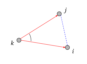
Formula (3.7) is the cosine theorem for a triangle. Here the pairs between which the mutual norm is defined have a common element k - adjacent pairs.
Three scalar products can be defined on 3 vertices. Their sum is expressed in terms of the sum of the distances between the vertices:
The square of the scalar product on 3 vertices is related to the area of the triangle formed by them (Heron's formula):
In the general case, the vertices of the pairs may not lie in the same plane, therefore, this definition of the scalar product cannot always be associated with the cosine of the angle between the directions.
We list the properties of the scalar product (3.6).
1) Does not depend on the permutation of pairs:
2) Antisymmetric with respect to permutation of elements in a pair or :
3) For 4 elements there are only two independent scalar products of pairs due to the identity:
Mathematicians will see in formula (3.9.3) the first Bianchi identity . From which it can be concluded that the structures of the curvature tensor (Riemann) and the scalar product of pairs are similar.
4) The rate of independent pairs can be expressed in terms of the difference between the rates of adjacent pairs:
We will use this identity in the next article.
5) Distance between elements and can be expressed in terms of the scalar products of adjacent and independent pairs:
As the elements forming a pair, the vertices of the base can be chosen. Then the scalar product of pairs becomes a tensor - a set of scalar products between all possible pairs of elements of a given basis. To distinguish tensors from scalars, we will use capital letters for the first ones. That is, instead of a scalar for the basis elements, we obtain the tensor .
The scalar product of pairs formed by elements of the basis can be expressed in terms of the properties of the Laplacian of the basis.
If two pairs of vertices are given and , the value of their scalar product can be obtained by dividing the cofactor of the 2nd order on the scalar potential of the laplacian :
Cofactor is called the determinant of the minor of a square matrix (taking into account the sign). Scalar potential - this is a cofactor of the 1st order from the Laplacian (see (1.12) from the first article ).
Thus, it is necessary to remove the columns corresponding to one vector from the Laplacian matrix (in the formula, this th columns), and rows corresponding to another ( ), after which the determinant of the resulting minor is divided by the scalar potential . If the deleted columns and rows of the Laplacian are the same, then we obtain the value of the distance between the nodes.
Between any pairs of vertices of the graph, you can define their mutual norm - the scalar product. Since the graph is usually given by the Laplacian, the formula (3.10.1) can be used for the calculation.
Let, for example, be chosen as the generating vertices of two pairs - and . Then the scalar product between these pairs is given by formula (3.6):
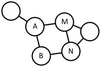
For a graph, which is an electrical circuit, the value of the scalar product reflects the concept of generalized resistance in an electrical circuit. To measure this (“apparent”) resistance, the current source (voltage) is applied to one node ( A and B ), and the potential difference is measured between the other ( M and N ). The mutual norm (scalar product) of pairs is equal to zero, if the external potential difference does not lead to the potential difference on the measured pair.
The graph does not have to be discrete, - the soil is an example of a solid (continuous) graph on which you can measure the scalar product between selected elements.

Installation scheme for the study of the resistance method: A and B - supply grounding; M and N - measuring grounding; 1 - measuring device (from the book "Electrical Prospecting", Yakubovsky Yu. B., M., 1980).
The figure shows the measurement scheme for the scalar product of pairs. and on the ground.
In the next article we will examine in more detail why the ratio of the given and measured potential differences of the nodes turned out to be associated with the scalar product of pairs.
A submatrix of values of mutual norms (scalar products) of pairs can be obtained by inverting the minor of the Laplacian. Denote the Laplacian from which removed row and th column as . Then the identity holds:
Note that in the matrix absent row and th column.
If the matrix of scalar products of pairs is known , then you can restore the distance matrix based on distance conversion. First we expand the submatrix missing line and column with zero values. Apply distance conversion to the resulting matrix:
which in our case takes the form of the identity (3.9.5):
The combination of formulas (3.10.2) and (3.10.3) is one of the ways to get the distance matrix for a given Laplacian. Remove any of the nodes from the Laplacian (let ) and pay. Get the matrix of scalar products of pairs (its other name is the fundamental matrix, see the next part). Index value fixed - base vertex. In the matrix the first vertex of the pairs is in the base node , and the second runs through the remaining vertices of the base.
Next, apply to the matrix distance conversion (3.10.3).
If in the graph to change the value of the conductivity of the edge (element of Laplacian), then it is obvious that all distances between the vertices will change (the norms of vectors) . With an increase in conductivity, the distances should decrease (decrease). The gift of the gods is that it is possible to estimate the change in distances not only qualitatively, but also quantitatively. Denote the derivative of the laplacian distance matrix as
Tensor Is the Jacobi matrix , that is, the expression of changes in the values of the distance matrix when changing the values of the laplacian . It turns out that this tensor is expressed in terms of the square of the scalar product of pairs:
That is, the change in the magnitude of the connection nodes leads to a change in the distance between the nodes proportional to the scalar product of pairs and .
Scalar product square tensor reversible. Imagine expression (3.11) in the following equivalent form:
This formula can be interpreted as a response. on impact . Tensor plays the role of transfer function (reaction to exposure).
It is also possible to reverse the situation in which the impact and response change places. Forward and reverse transfer functions are related by:
Good luck again - tensor can be expressed through the Laplacian:
Tensor values we call quadratic connectivity .
The values of the tensor are determined by the values of the Laplacian for 4 vertices. We consider these vertices as vertices of the graph. Suppose that all 4 vertices are different:
Here vectors denote pairs of vertices, between which quadratic connectivity is assumed. Couples have a non-zero quadroherence only when their vertices are pairwise connected (the necessary connections are shown in the figure in the same color). If all the connections in the graph are positive, then the quadratic connectivity between different vertices is also always greater or equal to zero.
If the pairs have a common vertex, then the sense of quad-connectivity changes. This is due to the fact that the diagonal elements of the Laplacian are not zero (as in the distance matrix), but reflect the common connectivity (conductivity) of the node.
Pairs of vertices may coincide - the diagonal elements of the quadratic connected tensor.
Here characterizes the connection of two nodes i and j . It is considered as the sum of the product of their total conductivity (degree of the top) and square connection between nodes .
Although it is formal for the tensor elements of the form can be calculated (one of the pairs is degenerate), the given (degenerate) elements are linearly dependent on the others. Can be calculated through the sum of the tensor for one of the indices of the pair:
___
Let's sum up. The concept of scalar product of pairs of elements that is useful in all respects is considered. In the next article we will work with the subspace of the graph - what it is and what its properties are.
Table of contents
Ordered pair
The coordinates of the vector can be obtained as the difference of the coordinates of the elements, but the reverse is not true - the coordinates of the elements forming it cannot be reconstructed from the coordinates of the vector. The coordinates of the two elements carry more information than the coordinates of the vector. Therefore, one can form a pair of elements - an improved analogue of the vector. Such a set of two elements is called an ordered pair .
Each ordered pair can be mapped a vector - the difference of the elements forming a pair. For two vectors, you can define the scalar product, which can also be considered as a characteristic of the four elements of space.
')
Scalar product
To reduce bulkiness in this part, we denote elements by lowercase characters. A pair is a combination of two elements: . The vector corresponding to the pair is the difference of the elements of the pair:
The element rate is its scalar product with itself:
The same definition can be used for the vector of a pair, which is known to reflect the square of the distance between the elements of the pair:
If two different pairs are given and then the scalar product can be defined between the corresponding vectors:
Indices ask one pair, and indexes - another.
Expression (3.4) defines a scalar depending on the relative position of the 4 elements. It is important that this scalar can be expressed in terms of the distances between the elements. .
As is known, the distance between the elements is associated with the scalar product between them:
.
Expanding the product (3.4) with (3.5) taken into account, we obtain:
This is the general formula for the scalar product of pairs. The order of the indices is important - it sets the pairs and the direction of the corresponding vectors.
Expressions like (3.6) often appear in different places in mathematics. This is due to the generality of the output of this formula. Note that we used only the most general properties of an algebraic expression. Therefore, any elements for which the product operation is defined can be used as elements. The identity will be true for them, in general form, it looks like this:
Couples with a common vertex - adjacent pairs
If couples have a common vertex , the formula (3.6) is simplified:
Formula (3.7) is the cosine theorem for a triangle. Here the pairs between which the mutual norm is defined have a common element k - adjacent pairs.
Three scalar products can be defined on 3 vertices. Their sum is expressed in terms of the sum of the distances between the vertices:
The square of the scalar product on 3 vertices is related to the area of the triangle formed by them (Heron's formula):
Independent pairs - four different peaks
In the general case, the vertices of the pairs may not lie in the same plane, therefore, this definition of the scalar product cannot always be associated with the cosine of the angle between the directions.
We list the properties of the scalar product (3.6).
1) Does not depend on the permutation of pairs:
2) Antisymmetric with respect to permutation of elements in a pair or :
3) For 4 elements there are only two independent scalar products of pairs due to the identity:
Mathematicians will see in formula (3.9.3) the first Bianchi identity . From which it can be concluded that the structures of the curvature tensor (Riemann) and the scalar product of pairs are similar.
4) The rate of independent pairs can be expressed in terms of the difference between the rates of adjacent pairs:
We will use this identity in the next article.
5) Distance between elements and can be expressed in terms of the scalar products of adjacent and independent pairs:
Pairs on the basis elements
As the elements forming a pair, the vertices of the base can be chosen. Then the scalar product of pairs becomes a tensor - a set of scalar products between all possible pairs of elements of a given basis. To distinguish tensors from scalars, we will use capital letters for the first ones. That is, instead of a scalar for the basis elements, we obtain the tensor .
Scalar Product and Laplacian Cofactors
The scalar product of pairs formed by elements of the basis can be expressed in terms of the properties of the Laplacian of the basis.
If two pairs of vertices are given and , the value of their scalar product can be obtained by dividing the cofactor of the 2nd order on the scalar potential of the laplacian :
Cofactor is called the determinant of the minor of a square matrix (taking into account the sign). Scalar potential - this is a cofactor of the 1st order from the Laplacian (see (1.12) from the first article ).
Thus, it is necessary to remove the columns corresponding to one vector from the Laplacian matrix (in the formula, this th columns), and rows corresponding to another ( ), after which the determinant of the resulting minor is divided by the scalar potential . If the deleted columns and rows of the Laplacian are the same, then we obtain the value of the distance between the nodes.
Dot scalar product on a graph
Between any pairs of vertices of the graph, you can define their mutual norm - the scalar product. Since the graph is usually given by the Laplacian, the formula (3.10.1) can be used for the calculation.
Let, for example, be chosen as the generating vertices of two pairs - and . Then the scalar product between these pairs is given by formula (3.6):
For a graph, which is an electrical circuit, the value of the scalar product reflects the concept of generalized resistance in an electrical circuit. To measure this (“apparent”) resistance, the current source (voltage) is applied to one node ( A and B ), and the potential difference is measured between the other ( M and N ). The mutual norm (scalar product) of pairs is equal to zero, if the external potential difference does not lead to the potential difference on the measured pair.
The graph does not have to be discrete, - the soil is an example of a solid (continuous) graph on which you can measure the scalar product between selected elements.
Installation scheme for the study of the resistance method: A and B - supply grounding; M and N - measuring grounding; 1 - measuring device (from the book "Electrical Prospecting", Yakubovsky Yu. B., M., 1980).
The figure shows the measurement scheme for the scalar product of pairs. and on the ground.
In the next article we will examine in more detail why the ratio of the given and measured potential differences of the nodes turned out to be associated with the scalar product of pairs.
The appeal of the minor laplacian
A submatrix of values of mutual norms (scalar products) of pairs can be obtained by inverting the minor of the Laplacian. Denote the Laplacian from which removed row and th column as . Then the identity holds:
Note that in the matrix absent row and th column.
If the matrix of scalar products of pairs is known , then you can restore the distance matrix based on distance conversion. First we expand the submatrix missing line and column with zero values. Apply distance conversion to the resulting matrix:
which in our case takes the form of the identity (3.9.5):
The combination of formulas (3.10.2) and (3.10.3) is one of the ways to get the distance matrix for a given Laplacian. Remove any of the nodes from the Laplacian (let ) and pay. Get the matrix of scalar products of pairs (its other name is the fundamental matrix, see the next part). Index value fixed - base vertex. In the matrix the first vertex of the pairs is in the base node , and the second runs through the remaining vertices of the base.
Next, apply to the matrix distance conversion (3.10.3).
Square dot product, Jacobi matrix
If in the graph to change the value of the conductivity of the edge (element of Laplacian), then it is obvious that all distances between the vertices will change (the norms of vectors) . With an increase in conductivity, the distances should decrease (decrease). The gift of the gods is that it is possible to estimate the change in distances not only qualitatively, but also quantitatively. Denote the derivative of the laplacian distance matrix as
Tensor Is the Jacobi matrix , that is, the expression of changes in the values of the distance matrix when changing the values of the laplacian . It turns out that this tensor is expressed in terms of the square of the scalar product of pairs:
That is, the change in the magnitude of the connection nodes leads to a change in the distance between the nodes proportional to the scalar product of pairs and .
Vertex quadroconnection tensor
Scalar product square tensor reversible. Imagine expression (3.11) in the following equivalent form:
This formula can be interpreted as a response. on impact . Tensor plays the role of transfer function (reaction to exposure).
It is also possible to reverse the situation in which the impact and response change places. Forward and reverse transfer functions are related by:
Good luck again - tensor can be expressed through the Laplacian:
Tensor values we call quadratic connectivity .
Quadjunction Tensor Properties
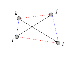
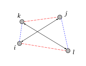
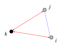
The values of the tensor are determined by the values of the Laplacian for 4 vertices. We consider these vertices as vertices of the graph. Suppose that all 4 vertices are different:
Here vectors denote pairs of vertices, between which quadratic connectivity is assumed. Couples have a non-zero quadroherence only when their vertices are pairwise connected (the necessary connections are shown in the figure in the same color). If all the connections in the graph are positive, then the quadratic connectivity between different vertices is also always greater or equal to zero.
If the pairs have a common vertex, then the sense of quad-connectivity changes. This is due to the fact that the diagonal elements of the Laplacian are not zero (as in the distance matrix), but reflect the common connectivity (conductivity) of the node.
Pairs of vertices may coincide - the diagonal elements of the quadratic connected tensor.
Here characterizes the connection of two nodes i and j . It is considered as the sum of the product of their total conductivity (degree of the top) and square connection between nodes .
Although it is formal for the tensor elements of the form can be calculated (one of the pairs is degenerate), the given (degenerate) elements are linearly dependent on the others. Can be calculated through the sum of the tensor for one of the indices of the pair:
___
Let's sum up. The concept of scalar product of pairs of elements that is useful in all respects is considered. In the next article we will work with the subspace of the graph - what it is and what its properties are.
Source: https://habr.com/ru/post/338762/
All Articles