On the classification of Fourier transform methods by examples of their software implementation by means of Python
Introduction
Publications by the Fourier method can be divided into two groups. The first group of so-called educational publications, for example, [1,2].
The second group of publications concerns the application of Fourier transforms in engineering, for example, during spectral analysis [3,4].
In no case, without begging the merits of these groups of publications, it is necessary to recognize that without classification, or at least attempts to implement such a classification, to get a systematic idea of the Fourier method, in my opinion, is difficult.
')
Publishing tasks
To classify Fourier transform methods using examples of their software implementation using Python tools. At the same time, to facilitate reading, use formulas only in the program code with corresponding explanations.
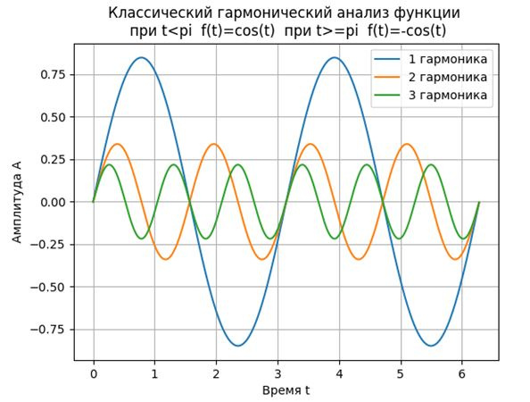
Harmonic analysis and synthesis
Harmonic analysis is the expansion of the function f (t) given on the interval [0, T] in a Fourier series or in the calculation of the Fourier coefficients by the formulas.
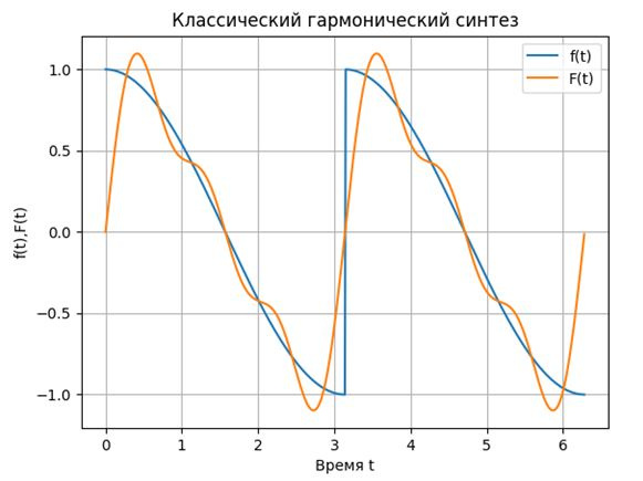
Harmonic synthesis is called obtaining vibrations of complex shape by summing up their harmonic components (harmonics).
Software implementation
#!/usr/bin/python # -*- coding: utf-8 -* from scipy.integrate import quad # import matplotlib.pyplot as plt # import numpy as np # T=np.pi; w=2*np.pi/T# def func(t):# if t<np.pi: p=np.cos(t) else: p=-np.cos(t) return p def func_1(t,k,w):# a[k] if t<np.pi: z=np.cos(t)*np.cos(w*k*t) else: z=-np.cos(t)*np.cos(w*k*t) return z def func_2(t,k,w):# b[k] if t<np.pi: y=np.cos(t)*np.sin(w*k*t) else: y=-np.cos(t)*np.sin(w*k*t) return y a=[];b=[];c=4;g=[];m=np.arange(0,c,1);q=np.arange(0,2*np.pi,0.01)# a=[round(2*quad(func_1, 0, T, args=(k,w))[0]/T,3) for k in m]# a[k], k - b=[round(2*quad(func_2, 0, T, args=(k,w))[0]/T,3) for k in m]# b[k], k - F1=[a[1]*np.cos(w*1*t)+b[1]*np.sin(w*1*t) for t in q]# F2=[a[2]*np.cos(w*2*t)+b[2]*np.sin(w*2*t) for t in q] F3=[a[3]*np.cos(w*3*t)+b[3]*np.sin(w*3*t) for t in q] plt.figure() plt.title(" \n t<pi f(t)=cos(t) t>=pi f(t)=-cos(t)") plt.plot(q, F1, label='1 ') plt.plot(q, F2 , label='2 ') plt.plot(q, F3, label='3 ') plt.xlabel(" t") plt.ylabel(" ") plt.legend(loc='best') plt.grid(True) F=np.array(a[0]/2)+np.array([0*t for t in q-1])# a[0]/2 for k in np.arange(1,c,1): F=F+np.array([a[k]*np.cos(w*k*t)+b[k]*np.sin(w*k*t) for t in q])# plt.figure() P=[func(t) for t in q] plt.title(" ") plt.plot(q, P, label='f(t)') plt.plot(q, F, label='F(t)') plt.xlabel(" t") plt.ylabel("f(t),F(t)") plt.legend(loc='best') plt.grid(True) plt.show() Result
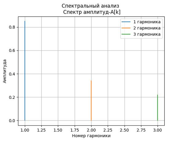
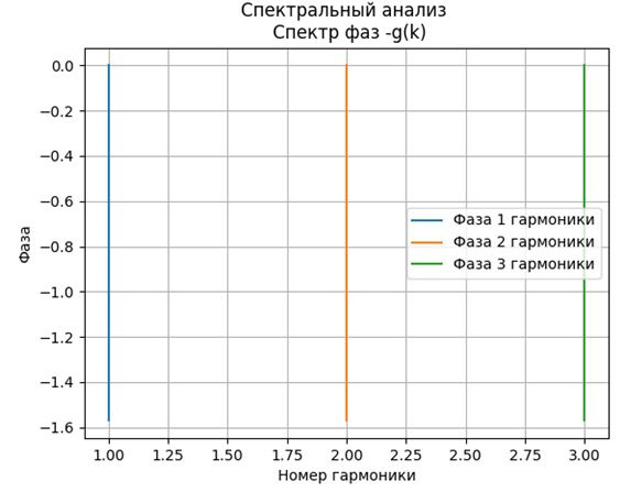
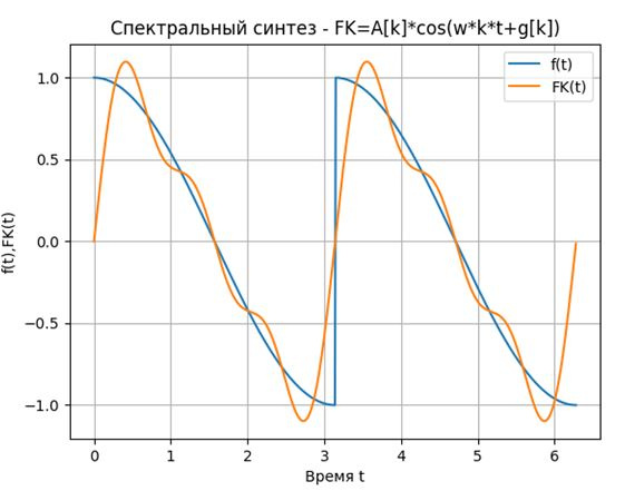
The spectral analysis of periodic functions consists in finding the amplitude Ak and the phase jk of the harmonics (cosine) of the Fourier series. The inverse problem of spectral analysis is called spectral synthesis .
Software implementation for spectral analysis and synthesis without special NumPy functions for Fourier transform
#!/usr/bin/python # -*- coding: utf-8 -* from scipy.integrate import quad # import matplotlib.pyplot as plt # import numpy as np # T=np.pi; w=2*np.pi/T# def func(t):# if t<np.pi: p=np.cos(t) else: p=-np.cos(t) return p def func_1(t,k,w):# a[k] if t<np.pi: z=np.cos(t)*np.cos(w*k*t) else: z=-np.cos(t)*np.cos(w*k*t) return z def func_2(t,k,w):# b[k] if t<np.pi: y=np.cos(t)*np.sin(w*k*t) else: y=-np.cos(t)*np.sin(w*k*t) return y a=[];b=[];c=4;g=[];m=np.arange(0,c,1);q=np.arange(0,2*np.pi,0.01)# a=[round(2*quad(func_1, 0, T, args=(k,w))[0]/T,3) for k in m]# a[k], k - b=[round(2*quad(func_2, 0, T, args=(k,w))[0]/T,3) for k in m]# b[k], k - plt.figure() plt.title(" \n -A[k]") A=np.array([(a[k]**2+b[k]**2)**0.5 for k in m])# plt.plot([m[1],m[1]],[0,A[1]],label='1 ') plt.plot([m[2],m[2]],[0,A[2]],label='2 ') plt.plot([m[3],m[3]],[0,A[3]],label='3 ') plt.xlabel(" ") plt.ylabel("") plt.legend(loc='best') plt.grid(True) for k in m:# if a[k]!=0: g.append(-np.tanh(b[k]/a[k])) else: g.append(-np.pi/2)# plt.figure() plt.title(" \n -g(k)") plt.plot([m[1],m[1]],[0, g[1]],label=' 1 ') plt.plot([m[2],m[2]],[0, g[2]],label=' 2 ') plt.plot([m[3],m[3]],[0, g[3]],label=' 3 ') plt.xlabel(" ") plt.ylabel("") plt.legend(loc='best') plt.grid(True) plt.figure() plt.title(" - FK=A[k]*cos(w*k*t+g[k])") FK=-np.array(a[0]/2)+np.array([0*t for t in q-1])# for k in m: FK=FK+np.array([A[k]*np.cos(w*k*t+g[k]) for t in q])# P=[func(t) for t in q] plt.plot(q, P, label='f(t)') plt.plot(q, FK, label='FK(t)') plt.xlabel(" t") plt.ylabel("f(t),FK(t)") plt.legend(loc='best') plt.grid(True) plt.show() Result
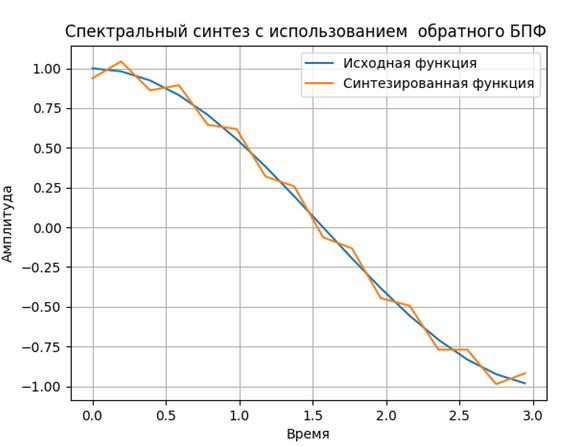
Software implementation of spectral analysis and synthesis using the NumPy functions of the forward fast Fourier transform - rfft and the inverse transform - irfft
#!/usr/bin/python # -*- coding: utf-8 -* import matplotlib.pyplot as plt import numpy as np import numpy.fft T=np.pi;z=T/16; m=[k*z for k in np.arange(0,16,1)];arg=[];q=[]# 16 def f(t):# if t<np.pi: p=np.cos(t) else: p=-np.cos(t) return p v=[f(t) for t in m] F=np.fft.rfft(v, n=None, axis=-1) # A=[((F[i].real)**2+(F[i].imag)**2)**0.5 for i in np.arange(0,7,1)]# for i in np.arange(0,7,1):# if F[i].imag!=0: t=(-np.tanh((F[i].real)/(F[i].imag))) arg.append(t) else: arg.append(np.pi/2) plt.figure() plt.title(" ") plt.plot(np.arange(0,7,1),arg,label='') plt.plot(np.arange(0,7,1),A,label='') plt.xlabel("") plt.ylabel(",") plt.legend(loc='best') plt.grid(True) for i in np.arange(0,9,1): if i<=7: q.append(F[i]) else: q.append(0) h=np.fft.irfft(q, n=None, axis=-1)# plt.figure() plt.title(" ") plt.plot(m, v,label=' ') plt.plot(m, h,label=' ') plt.xlabel("") plt.ylabel("") plt.legend(loc='best') plt.grid(True) plt.show() 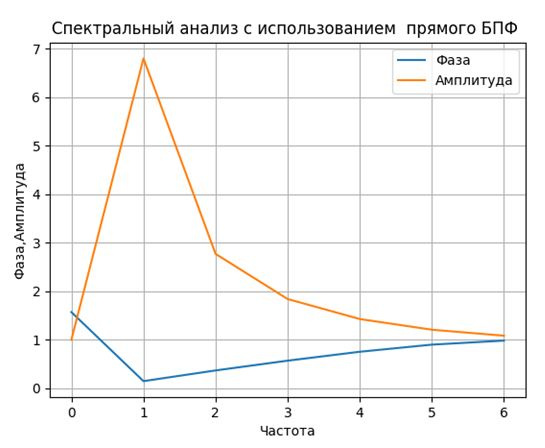
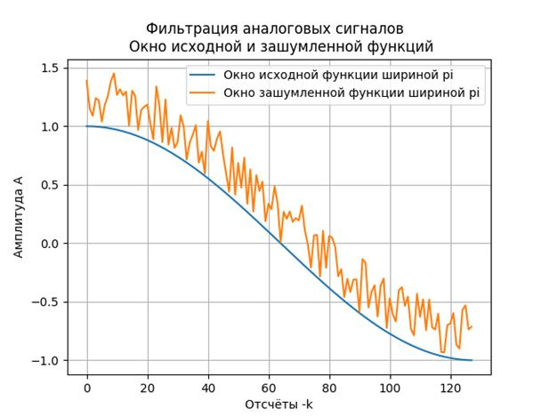
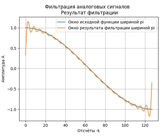
Analog signal filtering
By filtering is meant the selection of a useful signal from its mixture with an interfering signal — noise. The most common type of filtering is frequency filtering. If the region of frequencies occupied by the useful signal is known, it is sufficient to select this region and suppress those regions that are occupied by noise.
The software implementation illustrates the FFT filtering technique. First, the source signal is synthesized, represented by 128 samples of the vector v. Then noise is added to this signal using a random number generator (np. Random.uniform (0.0.5) function) and a vector of 128 samples of the noisy signal is formed.
Software implementation
#!/usr/bin/python # -*- coding: utf-8 -* import matplotlib.pyplot as plt import numpy as np from numpy.fft import rfft, irfft from numpy.random import uniform k=np.arange(0,128,1) T=np.pi;z=T/128; m=[t*z for t in k]# 128 def f(t):# if t<np.pi: p=np.cos(t) else: p=-np.cos(t) return p def FH(x):# if x>=0: q=1 else: q=0 return q v=[f(t) for t in m]# vs= [f(t)+np.random.uniform(0,0.5) for t in m]# plt.figure() plt.title(" \n ") plt.plot(k,v, label=' pi') plt.plot(k,vs,label=' pi') plt.xlabel(" -k") plt.ylabel(" ") plt.legend(loc='best') plt.grid(True) al=2# fs=np. fft.rfft(v)# g=[fs[j]*FH(abs(fs[j])-2) for j in np.arange(0,65,1)]# h=np.fft.irfft(g) # plt.figure() plt.title(" \n ") plt.plot(k,v,label=' pi') plt.plot(k,h, label=' pi') plt.xlabel(" -k") plt.ylabel(" ") plt.legend(loc='best') plt.grid(True) plt.show() Result
Solving partial differential equations
The algorithm for solving differential equations of mathematical physics using direct and inverse FFT is given in [5]. We use the above data for a software implementation in Python of solving a differential equation of heat propagation in a rod using the Fourier transform.
Software implementation
#!/usr/bin/env python #coding=utf8 import numpy as np from numpy.fft import fft, ifft # import pylab# from mpl_toolkits.mplot3d import Axes3D# n=50# 2 50 times=10# h=0.01# x=[r*2*np.pi/n for r in np.arange(0,n)]# w= np.fft.fftfreq(n,0.02)# k2=[ r**2 for r in w]# u0 =[2 +np.sin(i) + np.sin(2*i) for i in x]# u = np.zeros([times,n])# 10*50 u[0,:] = u0 # uf =np.fft. fft(u0) # for i in np.arange(1,times,1): uf=uf*[(1-h*k) for k in k2] # u[i,:]=np.fft.ifft(uf).real # X = np.zeros([times,n])# for i in np.arange(0,times,1): X[i:]=x T = np.zeros([times,n])# t for i in np.arange(0,times,1): T[i:]=[h*i for r in np.arange(0,n)] fig = pylab.figure() axes = Axes3D(fig) axes.plot_surface(X, T, u) pylab.show() Result

Conclusion
The article presents an attempt to classify by the areas of application of the Fourier transform methods.
Links
Source: https://habr.com/ru/post/338704/
All Articles