MVP recommendation system for GitHub weekly

Recall just in case someone has forgotten that GitHub is one of the largest software development platforms and home to many popular open source projects. On the “ Explore ” GitHub page, you can find information about projects that are gaining popularity, projects that people like you have subscribed to, as well as popular projects that are combined in areas or programming languages.

What you will not find is personal recommendations of projects based on your activity. This is somewhat surprising, since users put a huge number of stars to various projects on a daily basis, and this information can be easily used to build recommendations.

In this article, we share our experience building a recommendation system for GitHub from idea to implementation.

Idea

Every GitHub user can put a star to a project he likes. Having information about how each user has put stars in the repositories, we can find similar users and recommend them to pay attention to projects that they may not have seen yet, but who have already liked users with similar tastes. The scheme works in the opposite direction: we can find projects that are similar to those that the user already liked, and recommend them to him.

In other words, the idea can be formulated as follows: get data about users and the stars that they set, apply collaborative filtering methods to this data and wrap everything in a web application, with the help of recommendations will be available to end users.

We collect data

GHTorrent is a great project that collects data obtained using the public GitHub API and provides access to them in view of the monthly MySQL dumps. These dumps can be found in the “ Downloads ” section of the GHTorrent site.

Inside each dump you can find a SQL file with a description of the database schema, as well as several CSV files with data from the tables. As we said in the previous section, our approach is based on collaborative filtering. This approach implies that we need information about users and their preferences, or, to paraphrase this in terms of GitHub, about the users and the stars that they put on different projects.

Fortunately, the mentioned dumps contain all the necessary information in the following files:

• watchers.csv contains a list of repositories and users who gave them stars
• users.csv contains a pair of user id and username on GitHub
• projects.csv does the same for projects.

Let's look at the data more closely. Below is the beginning of the file watchers.csv (column names have been added for convenience):

You can see that users with id = 1, 2, 4, 6, 7, liked the project with id = 1 ... We do not need a column with a timestamp.

Not a bad start, but before moving on to building a model, it would be nice to look at the data more closely and possibly clean it up.

Research data

An interesting question that immediately comes to mind is: “How many stars did each user put on average?” A histogram showing the number of users who put different numbers of stars is shown below:

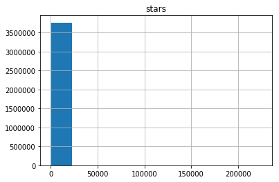
Hmm ... It doesn't look very informative. It seems that the absolute majority of users put a very small number of stars, but some users put them more than 200 thousand (wow!). Data visualization below confirms our assumptions:

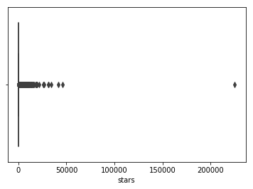
It all fits: one of the users has put more than 200 thousand stars. We also see a large amount of emissions - users with more than 25 thousand stars. Before continuing, let's see who this user is with 200 thousand stars. Meet our hero - user with the nickname 4148 . At the time of this writing, the page returns error 404. Silver medalist in the number of stars put - a user with the “talking” name StarTheWorld with 46 thousand stars (the page also returns a 404th error).

Now it is clear that the variable is subject to an exponential distribution (finding its parameters can be an interesting task). An important observation is that about half of the users rated less than five projects. This observation will be useful when we start modeling.

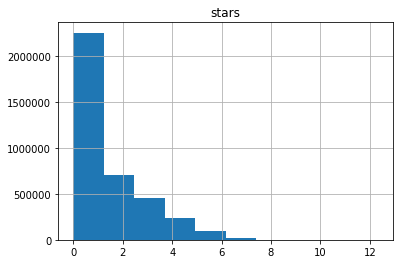
Let's turn to the repositories and take a look at the distribution of the number of stars:

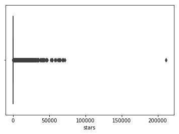
As in the case of users, we have one very noticeable outlier - the freeCodeCamp project with more than 200 thousand stars!

The histogram of the random number of stars in the repository after a logarithmic transformation is shown below and shows that we are again dealing with an exponential distribution, but with a sharper descent. As you can see, only a small part of the repositories has more than ten stars.

Preliminary data processing

To understand what data manipulations we need to do, we need to more closely familiarize ourselves with the collaborative filtering method that we are going to use.

Most collaborative filtering algorithms are based on matrix factorization and factorize user preference matrices. In the course of factorization are hidden characteristics of the products and the user's reaction to them. Knowing the parameters of a product that the user has not yet appreciated, we can predict his reaction based on his preferences.

In our case, we have a mxn matrix, where each row represents a user, and each column is a repository. r_ij is equal to one if the i th user has set a star to the j -th repository.

The R matrix can be easily built using the watchers.csv file. However, let us remember that most users put very few stars! What information about user preferences can we find out with so little information? In fact, no. It is very difficult to make assumptions about someone's tastes, knowing only one subject that you like.

At the same time, “one-star” users can significantly affect the predictive power of the model, introducing unjustified noise. Therefore, it was decided to exclude users about whom we have little information. Experiments have shown that excluding users with less than thirty stars gives good results. For excluded users, recommendations are based on the popularity of projects, which gives a good result.

Evaluation of the effectiveness of the model

Let's now discuss the important issue of model performance evaluation. We used the following metrics:

• accuracy and completeness (precision and recall)
• root mean square error (RMSE)

and came to the conclusion that the metric “accuracy-completeness” does not help much in our case.

But before we begin, it makes sense to mention another simple and effective method of evaluating effectiveness - building recommendations for ourselves and a subjective assessment of how good they are. Of course, this is not the method that you want to mention in your doctoral dissertation, but it helps to avoid mistakes in the early stages. For example, building recommendations for yourself using the full set of data showed that the resulting recommendations are not entirely relevant. Relevance increased significantly after the removal of users with a small number of stars.

Again we turn to the metric "accuracy-completeness." In simple terms, the accuracy of a model that predicts one of two possible outcomes is the ratio of the number of true-positive predictions to the total number of predictions. This definition can be written as a formula:

Thus, the accuracy is the number of hits in the target to the total number of attempts.

Completeness is the ratio of the number of true-positive predictions to the number of positive examples in all data:

In terms of our task, accuracy can be defined as the ratio of the repositories in the recommendations that the user assigned the stars to. Unfortunately, this metric does not give us much, since our goal is to predict not what the user has already appreciated, but what he will most likely appreciate. It may happen that some projects have a set of parameters that make them good candidates for the role of the following projects that the user likes, and the only reason why the user did not rate them is that he has not seen them yet.

We can modify this metric in order to make it useful: if we could measure how many of the recommended projects the user would later rate and divide it by the number of recommendations issued, then we would get a more accurate value of accuracy. However, at the moment we are not collecting any feedback, so accuracy is not the metric we would like to use.

Completeness, with reference to our task, is the ratio of the number of repositories in the recommendations that the user assigned the stars to the number of all repositories rated by the user. As with precision, this metric is not very useful, because the number of repositories in the recommendations is fixed and quite small (100 at the moment), and the value for accuracy is close to zero for users who rate a large number of projects.

Taking into account the thoughts presented above, it was decided to use the standard deviation as the main metric for assessing the effectiveness of the model. In terms of our problem, a metric can be written like this:

In other words, we measure the rms error between the project’s user rating (0 and 1) and the predicted rating, which will be close to 1 for repositories that, according to the model, the user will rate. Note that w is 0 for all r_ij = 0 .

Putting it all together - modeling

As already mentioned, our recommendation system is based on matrix factorization, or rather on the alternating least squares (ALS) algorithm. It should be noted that according to our experiments, any matrix factorization algorithm will also work (SVD, NNMF).

ALS implementations are available in many machine-learning software packages (see, for example, the implementation for Apache Spark ). The algorithm attempts to decompose the original mxn matrix into the product of two mxk and nxk matrices:

The parameter k determines the number of “hidden” project parameters that we are trying to find. The k value affects the performance of the model. The value of k should be selected using cross-validation. The graph below shows the dependence of the RMSE value on the k value on the test dataset. A value k=12 looks like an optimal choice, therefore it was used for the final model.

Let's summarize and look at the resulting sequence of actions:

1. We load data from the watchers.csv file and delete all users who evaluated less than 30 projects.
2. We divide the data into training and test kits.
3. We select the parameter k using RMSE and test data.
4. We train the model on the combined data set using ALS with the number of factors = k .

Having a model that suits us, we can begin to discuss how to make it available to end users. In other words, how to build a web application around it.

Backend

Here is a list of what our backend should be able to do:

• GitHub authorization to get usernames
• REST API for sending requests like "give me 100 recommendations for a user with nick X"
• Collect information about user subscriptions for updates

Since we wanted to do everything quickly and simply, the choice fell on the following technologies: Django, Django REST framework, React.

In order to correctly process requests, it is necessary to store some data received from GHTorrent. The main reason is that GHTorrent uses its own user IDs that are not the same as GitHub IDs. Thus, we need to keep a pair of user id <-> user GitHub name . The same goes for repositories.

Since the number of users and repositories is large enough (20 and 64 million, respectively) and we did not want to spend a large amount of money on infrastructure, it was decided to try a “new” type of storage with compression in MongoDB .

So, we have two collections in MongoDB: users and projects .

Documents from the users collection look like this:

 { "_id": 325598, "login": "yurtaev" } 

and indexed by the login field to speed up the processing of requests.

An example of a document from the projects collection is shown below:

 { "_id": 32415, "name": "FreeCodeCamp/FreeCodeCamp", "description": "The https://freeCodeCamp.org open source codebase and curriculum. Learn to code and help nonprofits." }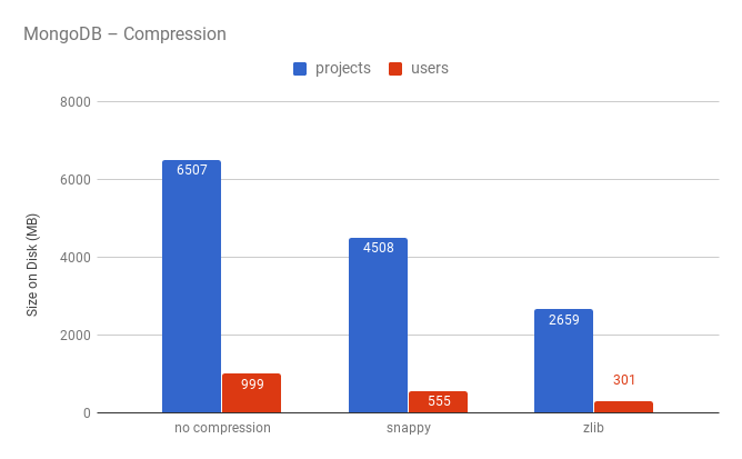 

As you can see, zlib compression gives us a twofold gain in terms of disk usage. One of the concerns associated with the use of compression was the speed of processing requests, but experiments have shown that time varies within the limits of statistical error. More information about the effect of compression on performance can be found here .

Summarizing, we can say that the compression in MongoDB gives a significant gain in terms of disk usage. Another advantage is the ease of scaling - it will be very useful when the amount of data on repositories and users will no longer fit on one server.

Model in action

There are two approaches to using the model:

1. Pre-generate recommendations for each user and save them to the database.
2. Generate recommendations on request.

The advantage of the first approach is that the model will not be a bottleneck (at the moment, the model can process from 30 to 300 requests for recommendations per second). The main drawback is the amount of data that needs to be stored. There are 20 million users. If we keep 100 recommendations for each user, it will result in 2 billion records! By the way, most of these 20 million users will never use the service, which means that most of the data will be stored just like that. Last but not least, building recommendations takes time.

Advantages and disadvantages of the second approach - mirroring the advantages and disadvantages of the first approach. But what we like in building recommendations on request is flexibility. The second approach allows you to return any number of recommendations that we need, and also makes it easy to replace the model.

After weighing all the pros and cons, we chose the second option. The model was packaged in a Docker container, and returns recommendations using an RPC call.

Frontend

Nothing super interesting: React , Create React App and Semantic UI . The only trick - React Snapshot was used to pre-generate a static version of the main page of the site for better indexing by search engines.

useful links

If you are a GitHub user, then you can get your recommendations on the GHRecommender website. Please note that if you rate less than 30 repositories, you will receive the most popular projects as recommendations.

GHRecommender sources are available here .

✎ Co-author of the text and project avli