How to distinguish birds from flowers. Or flowers from birds
As a weekend program, I wanted to play around with a kind of “neural” network (a spoiler - there are no neurons in it). And so that it would not be painfully painful for hours spent aimlessly, I thought that we feed him in vain, let him benefit, let this grid disassemble the home photo archive and at least arrange the photos of flowers into a separate folder.
 The simplest network was found in the article " Neural network in 11 lines in Python " (this is a translation from SLY_G of the article " A Neural Network in 11 lines of Python (Part 1) ", in general the author has another continuation " A Neural Network in 13 lines of Python (Part 2 - Gradient Descent) ", but the first article is enough here).
Brief description of the grid - there is exactly one dependency in this network - NumPy .
')
The set of inputs is treated as a matrix. , multiple outputs - as a vector . In the original article, the network multiplies the input matrix, in dimension (4 x 3), by the input weights matrix. (3 x 4), applies the transfer function to the product, and gets the layer matrix (4 x 4).
Next layer multiplied by the output weights matrix (4 x 1), is also passed through the function, and a layer is obtained (4 x 1), which is the result of the network.
Therefore, I have slightly modified the code from the article, added the transposition after multiplication and work with an arbitrary number of layers in the grid. This gave me the opportunity to receive any combination of dimensions of inputs and outputs.
For example, if it is necessary to have a matrix (3 x 4) at the input, and the output is a single number, then we add two matrices of synapses (4 x 1) and (3 x 1):
The resulting code is:
So, there is a grid, now you need to figure out how to load photos. Photos are on disk, mostly in JPG, but there are other formats. Their sizes are also different, depending on what they were shooting and how they were processed, from 3 Mpx to 16 Mpx.
At first I tried to upload photos via Qt, a QImage class, it can work with different formats, provides conversion and gives direct access to the image data. Surely there is a simpler way in Python, but I didn’t have to figure it out with a QImage. In order for the network to work with a picture, it should be transferred to a monochrome image and reduced to a standard size.
To transfer to the grid, you need to convert the image to the numpy.ndarray matrix. QImage.bits () gives a pointer to image data, where each byte corresponds to a pixel. In NumPy, there was a function called recarray, capable of making an array of records from the buffer, and it has a view method, which we will make the numpy.ndarray matrix without copying the data.
The picture, although reduced, directly fed to the input of the network will be too costly - I have already said that the network does matrix multiplication, so even one training cycle will result in 400x400x400 = 64 million multiplications. Experts recommend using convolution . Wikipedia has a wonderful illustration of her work:

This animation shows that the dimension of the result is equal to the dimension of the original matrix. But I’ll simplify my life a bit, I’ll not move by pixels, but break the image into pieces the same size as the input matrix, and apply the grid to them one by one. In matrices, cutting a piece is quite simple:
The result of processing the pieces by the network is formed into a matrix of a smaller size; this matrix is transmitted to the input of the common network. That is, there will be two networks - the first one works with pieces of the image, the second one with the result of the first network working on the pieces.
Creating a primary network:
Inside, self.net is created - the network itself, with the given size of the input shape matrix and with the output as an 1x1 elementary matrix. Yes, it was possible to inherit from the NN network class, but it was a holiday, I wanted to quickly get the result, but the architecture was not yet settled. Time to market beats in our hearts!
Image Counting by First Network:
At the output we have a resArr matrix, with a dimension equal to the number of pieces into which the image was divided. This matrix is passed to the input of the second network, which will give the final result.
Here you have to ask me where I took the first line, and what it means:
This is the expected result of the network in the event of a positive response, i.e. if the network believes that the input image of the flower. The dimension has chosen from the principle of “neither a little nor a lot” - if we take the dimension of 1x1, then it is difficult to judge from one resulting number how much the network “doubts” as a result. There is no sense to set a larger dimension too - it will not give more information. An equal number of zeros and ones gives a clear guideline - the closer to it, the greater the coincidence. If we take all the units or all the zeros, then the network will have an incentive to retrain - increase all factors or, accordingly, reset them to get the desired result regardless of the input data.
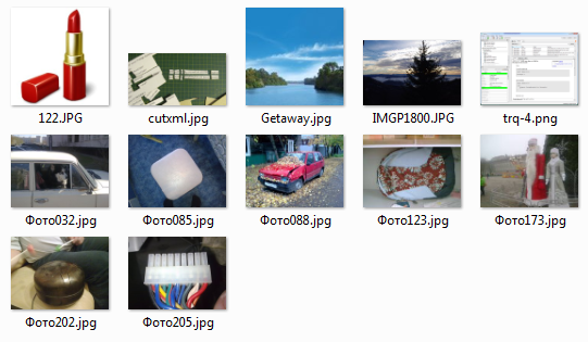
I made a training set of my own photos, simply expanding them into two catalogs:
flowers
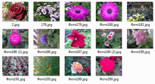
and noflowers
Paths to the pictures will collect in two arrays
Teaching simple networks is usually proposed, including in the original article, by the traditional method — the reverse propagation of error . But in order to apply this method to a convolutional network consisting of two elementary, it is necessary to ensure the end-to-end transmission of the accumulated error from the second network to the first. In general, there are other methods for convolutional networks. I was too lazy to redo the working network, at least for the time being, so I decided to train the second network, and not to train the first one at all, leave it crammed when creating random values, reasoning that since the human eye nerves are not trained, then I have nothing to teach the primary network, "Looking" at the image.
In each epoch, right after the training, I run the entire sample through the network and see what happened.
If the network has learned correctly, then at its output there should be a value close to the given [[1,0,1,0]], if there is a flower at the entrance, and as different as possible from the specified one, for example [[0,1,0, 1]], if the entrance is not a flower. The result is estimated, empirically I accepted a deviation from a successful result of no more than 0.2 - this is also a successful result, and the number of errors is considered. From all the runs, choose the one where the least errors are made, and save the weights of the synapses of both grids to files. Then these files can be used to load grids.
Hopefully, I launch and ... wait ..., then wait another ..., and also ... I get complete nonsense - the grid does not learn:
Being a carrier of real living, not artificial neurons, it dawned on me that the main difference between colors is color (yes, cap, thank you for being there, although you are often late with your advice). Therefore, it would be necessary to translate it into some color model, where the color component will be highlighted (HSV or HSL), and train the network on color.
But it turned out that the QImage class does not know such color spaces . I had to abandon it and upload photos using OpenCV, where such an opportunity exists.
True, OpenCV refused to work with Russian letters in file names, had to rename them.
Launched - the result is not pleased, almost the same.
I also thought, I decided that the problem was in very random values in the first grid, in vain I hoped that the stars would converge without my help, so I added a small pretraining to her, only 2 cycles per file. For a sample of a positive result, I took the identity matrix.
I started it again - it became much more interesting, the numbers began to change, although it did not reach the ideal.
Further ... And then the day off ended, and it was time for me to do household work.
Of course, this network, the way I taught it, and the test dataset correlate very little with real networks and what data scientists are doing. This is just a toy for gymnastics of the mind, do not place great hopes on it.
You can outline further steps on how to achieve the desired result (if you need one):
Continuation
The simplest network
The simplest network was found in the article " Neural network in 11 lines in Python " (this is a translation from SLY_G of the article " A Neural Network in 11 lines of Python (Part 1) ", in general the author has another continuation " A Neural Network in 13 lines of Python (Part 2 - Gradient Descent) ", but the first article is enough here).Brief description of the grid - there is exactly one dependency in this network - NumPy .
')
The set of inputs is treated as a matrix. , multiple outputs - as a vector . In the original article, the network multiplies the input matrix, in dimension (4 x 3), by the input weights matrix. (3 x 4), applies the transfer function to the product, and gets the layer matrix (4 x 4).
Next layer multiplied by the output weights matrix (4 x 1), is also passed through the function, and a layer is obtained (4 x 1), which is the result of the network.
Total, omitting the scalar transfer function, the network implements two matrix multiplications:
The consequence of this, according to the rules of matrix multiplication, is that one of the dimensions does not change during the operation of the network. and get at the output of a single number is impossible.
Therefore, I have slightly modified the code from the article, added the transposition after multiplication and work with an arbitrary number of layers in the grid. This gave me the opportunity to receive any combination of dimensions of inputs and outputs.
For example, if it is necessary to have a matrix (3 x 4) at the input, and the output is a single number, then we add two matrices of synapses (4 x 1) and (3 x 1):
Or, say, you can convert an input matrix (10 x 8) to an output (4 x 5):
The resulting code is:
nnmat.py
Result of work:
import numpy as np def nonlin(x,deriv=False): if(deriv==True): return (x)*(1-(x)) return 1/(1+np.exp(-x)) def fmax(x,deriv=False): if(deriv==True): return 0.33 return np.maximum(x,0)/3 class NN: def __init__(self, shapes, func=nonlin): self.func = func self.shapes = shapes self.syns = [ 2*np.random.random((shapes[i-1][1],shapes[i][0])) - 1 for i in range(1, len(shapes)) ] self.layers = [ np.zeros(shapes[i]) for i in range(1, len(shapes)) ] def learn(self, X, y, cycles): for j in range(cycles): res = self.calc(X) prev = y - res for i in range(len(self.layers)-1,-1,-1): l_delta = (prev*self.func(self.layers[i], True)).T if i == 0: self.syns[i] += XTdot(l_delta) else: prev = l_delta.dot(self.syns[i].T) self.syns[i] += self.layers[i-1].T.dot(l_delta) return self.layers[-1] def calc(self,X): for i in range(len(self.syns)): if i == 0: self.layers[i] = self.func(np.dot(X,self.syns[i])).T else: self.layers[i] = self.func(np.dot(self.layers[i-1],self.syns[i])).T return self.layers[-1] if __name__ == '__main__': X = np.array([ [0,0,1],[0,1,1],[1,0,1],[1,1,1] ]) y = np.array([[0,1,1,0]]) print('X =',X) print('y =',y) nn = NN((X.shape, (y.shape[1], X.shape[0]), y.shape)) nn.learn(X,y,1000) print('Result =',nn.calc(X).round(2)) Result of work:
X = [[0 0 1] [0 1 1] [1 0 1] [1 1 1]] y = [[0 1 1 0]] Result = [[ 0.02 0.99 0.98 0.02]] Upload photos
So, there is a grid, now you need to figure out how to load photos. Photos are on disk, mostly in JPG, but there are other formats. Their sizes are also different, depending on what they were shooting and how they were processed, from 3 Mpx to 16 Mpx.
At first I tried to upload photos via Qt, a QImage class, it can work with different formats, provides conversion and gives direct access to the image data. Surely there is a simpler way in Python, but I didn’t have to figure it out with a QImage. In order for the network to work with a picture, it should be transferred to a monochrome image and reduced to a standard size.
def readImage(file, imageSize): img = QImage(file) if img.isNull(): return 0 img = img.convertToFormat(QImage.Format_Grayscale8) img = img.scaled(imageSize[0],imageSize[1],Qt.IgnoreAspectRatio) return img To transfer to the grid, you need to convert the image to the numpy.ndarray matrix. QImage.bits () gives a pointer to image data, where each byte corresponds to a pixel. In NumPy, there was a function called recarray, capable of making an array of records from the buffer, and it has a view method, which we will make the numpy.ndarray matrix without copying the data.
srcBi = img.bits() srcBi.setsize(img.width() * img.height()) srcBy = bytes(srcBi) srcW, srcH = img.width(), img.height() srcArr = np.recarray((srcH, srcW), dtype=np.int8, buf=srcBy).view(dtype=np.byte,type=np.ndarray) Network for images
The picture, although reduced, directly fed to the input of the network will be too costly - I have already said that the network does matrix multiplication, so even one training cycle will result in 400x400x400 = 64 million multiplications. Experts recommend using convolution . Wikipedia has a wonderful illustration of her work:
This animation shows that the dimension of the result is equal to the dimension of the original matrix. But I’ll simplify my life a bit, I’ll not move by pixels, but break the image into pieces the same size as the input matrix, and apply the grid to them one by one. In matrices, cutting a piece is quite simple:
srcArr[x:x+dw, y:y+dw] The result of processing the pieces by the network is formed into a matrix of a smaller size; this matrix is transmitted to the input of the common network. That is, there will be two networks - the first one works with pieces of the image, the second one with the result of the first network working on the pieces.
Creating a primary network:
class ImgNN: def __init__(self, shape, resultShape = (16, 16), imageSize = (400,400)): self.resultShape = resultShape self.w = imageSize[0] // shape[0] self.h = imageSize[1] // shape[1] self.net = NN([shape, (1,shape[0]), (1,1)]) self.shape = shape self.imageSize = imageSize Inside, self.net is created - the network itself, with the given size of the input shape matrix and with the output as an 1x1 elementary matrix. Yes, it was possible to inherit from the NN network class, but it was a holiday, I wanted to quickly get the result, but the architecture was not yet settled. Time to market beats in our hearts!
Image Counting by First Network:
def calc(self, srcArr): w = srcArr.shape[0] // self.shape[0] h = srcArr.shape[1] // self.shape[1] resArr = np.zeros(self.resultShape) for x in range(w): for y in range(h): a = srcArr[x:x+self.shape[0], y:y+self.shape[1]] if a.shape != (self.shape[0], self.shape[1]): continue if x >= self.resultShape[0] or y >= self.resultShape[1]: continue res = self.nn.calc(a) resArr[x,y] = res[0,0] return resArr At the output we have a resArr matrix, with a dimension equal to the number of pieces into which the image was divided. This matrix is passed to the input of the second network, which will give the final result.
y = np.array([[1,0,1,0]]) firstShape = (40, 40) middleShape = (5, 5) imageSize = firstShape[0]*middleShape[0], firstShape[1]*middleShape[1] ... nn = ImgNN(firstShape, resultShape=middleShape, imageSize=imageSize) nn2 = NN([middleShape, (y.shape[1], middleShape[0]), y.shape]) ... i = readImage(f, imageSize) mid = nn.calc(i) res = nn2.calc(mid) Here you have to ask me where I took the first line, and what it means:
y = np.array([[1,0,1,0]]) This is the expected result of the network in the event of a positive response, i.e. if the network believes that the input image of the flower. The dimension has chosen from the principle of “neither a little nor a lot” - if we take the dimension of 1x1, then it is difficult to judge from one resulting number how much the network “doubts” as a result. There is no sense to set a larger dimension too - it will not give more information. An equal number of zeros and ones gives a clear guideline - the closer to it, the greater the coincidence. If we take all the units or all the zeros, then the network will have an incentive to retrain - increase all factors or, accordingly, reset them to get the desired result regardless of the input data.
How to train a convolutional network?
I made a training set of my own photos, simply expanding them into two catalogs:
flowers
and noflowers
Paths to the pictures will collect in two arrays
import os fl = [e.path for e in os.scandir('flowers')] nofl = [e.path for e in os.scandir('noflowers')] all = fl+nofl Teaching simple networks is usually proposed, including in the original article, by the traditional method — the reverse propagation of error . But in order to apply this method to a convolutional network consisting of two elementary, it is necessary to ensure the end-to-end transmission of the accumulated error from the second network to the first. In general, there are other methods for convolutional networks. I was too lazy to redo the working network, at least for the time being, so I decided to train the second network, and not to train the first one at all, leave it crammed when creating random values, reasoning that since the human eye nerves are not trained, then I have nothing to teach the primary network, "Looking" at the image.
for epoch in range(100): print('Epoch =', epoch) nn = ImgNN(firstShape, resultShape=middleShape, imageSize=imageSize) nn2 = NN([middleShape, (y.shape[1], middleShape[0]), y.shape]) for f in fl: i = readImage(f, imageSize) # nn.learn(i, yy, 1) mid = nn.calc(i) nn2.learn(mid, y, 1000) In each epoch, right after the training, I run the entire sample through the network and see what happened.
for f in all: i = readImage(f, imageSize) mid = nn.calc(i) res = nn2.calc(mid) delta = abs(y-res) v = round(np.std(delta),3) If the network has learned correctly, then at its output there should be a value close to the given [[1,0,1,0]], if there is a flower at the entrance, and as different as possible from the specified one, for example [[0,1,0, 1]], if the entrance is not a flower. The result is estimated, empirically I accepted a deviation from a successful result of no more than 0.2 - this is also a successful result, and the number of errors is considered. From all the runs, choose the one where the least errors are made, and save the weights of the synapses of both grids to files. Then these files can be used to load grids.
if v > 0.2 and f in fl: fails += 1 failFiles.append(f) elif v<0.2 and f in nofl: fails +=1 failFiles.append(f) if minFails == None or fails < minFails: minFails = fails lastSyns = nn.net.syns lastSyns2 = nn2.syns print('fails =',fails, failFiles) print('min =',minFails) if minFails <= 1: print('found!') break for i in range(len(lastSyns)): np.savetxt('syns_save%s.txt'%i, lastSyns[i]) for i in range(len(lastSyns2)): np.savetxt('syns2_save%s.txt'%i, lastSyns2[i]) Though call it a rose, though not
Hopefully, I launch and ... wait ..., then wait another ..., and also ... I get complete nonsense - the grid does not learn:
Nothing happened
flowers\178.jpg res = [[ 0.98 0.5 0.98 0.5 ]] v = 0.241
flowers\179.jpg res = [[ 0.98 0.5 0.98 0.5 ]] v = 0.24
flowers\180.jpg res = [[ 0.98 0.5 0.98 0.5 ]] v = 0.241
flowers\182.jpg res = [[ 0.98 0.5 0.98 0.5 ]] v = 0.24
flowers\186-2.jpg res = [[ 0.98 0.5 0.98 0.5 ]] v = 0.241
flowers\186.jpg res = [[ 0.98 0.5 0.98 0.5 ]] v = 0.24
flowers\187.jpg res = [[ 0.98 0.5 0.98 0.5 ]] v = 0.24
flowers\190 (2).jpg res = [[ 0.98 0.5 0.98 0.5 ]] v = 0.24
flowers\190.jpg res = [[ 0.98 0.5 0.98 0.5 ]] v = 0.241
flowers\191.jpg res = [[ 0.98 0.5 0.98 0.5 ]] v = 0.24
flowers\195.jpg res = [[ 0.98 0.5 0.98 0.5 ]] v = 0.241
flowers\199.jpg res = [[ 0.98 0.5 0.98 0.5 ]] v = 0.24
flowers\2.jpg res = [[ 0.98 0.5 0.98 0.5 ]] v = 0.241
flowers\200.jpg res = [[ 0.98 0.5 0.98 0.5 ]] v = 0.241
noflowers\032.jpg res = [[ 0.98 0.5 0.98 0.5 ]] v = 0.241
noflowers\085.jpg res = [[ 0.98 0.5 0.98 0.5 ]] v = 0.24
noflowers\088.jpg res = [[ 0.98 0.5 0.98 0.5 ]] v = 0.241
noflowers\122.JPG res = [[ 0.98 0.5 0.98 0.5 ]] v = 0.241
noflowers\123.jpg res = [[ 0.98 0.5 0.98 0.5 ]] v = 0.241
noflowers\173.jpg res = [[ 0.98 0.5 0.98 0.5 ]] v = 0.24
noflowers\202.jpg res = [[ 0.98 0.5 0.98 0.5 ]] v = 0.241
noflowers\205.jpg res = [[ 0.98 0.5 0.98 0.5 ]] v = 0.241
noflowers\cutxml.jpg res = [[ 0.98 0.5 0.98 0.5 ]] v = 0.241
noflowers\Getaway.jpg res = [[ 0.98 0.5 0.98 0.5 ]] v = 0.24
noflowers\IMGP1800.JPG res = [[ 0.98 0.5 0.98 0.5 ]] v = 0.24
noflowers\trq-4.png res = [[ 0.97 0.51 0.97 0.51]] v = 0.239
fails = 14
Being a carrier of real living, not artificial neurons, it dawned on me that the main difference between colors is color (yes, cap, thank you for being there, although you are often late with your advice). Therefore, it would be necessary to translate it into some color model, where the color component will be highlighted (HSV or HSL), and train the network on color.
But it turned out that the QImage class does not know such color spaces . I had to abandon it and upload photos using OpenCV, where such an opportunity exists.
import cv2 def readImageCV(file, imageSize): img = cv2.imread(file) small = cv2.resize(img, imageSize) hsv = cv2.cvtColor(small, cv2.COLOR_BGR2HSV) return hsv[:,:,0]/255 True, OpenCV refused to work with Russian letters in file names, had to rename them.
Launched - the result is not pleased, almost the same.
I also thought, I decided that the problem was in very random values in the first grid, in vain I hoped that the stars would converge without my help, so I added a small pretraining to her, only 2 cycles per file. For a sample of a positive result, I took the identity matrix.
yy = np.zeros(middleShape) np.fill_diagonal(yy,1) ... for f in fl: i = readImage(f, imageSize) nn.learn(i, yy, 2) # - mid = nn.calc(i) nn2.learn(mid, y, 1000) I started it again - it became much more interesting, the numbers began to change, although it did not reach the ideal.
Best result
Epoch = 34
flowers\178.jpg res = [[ 0.86 0.47 0.88 0.47]] v = 0.171
flowers\179.jpg res = [[ 0.87 0.51 0.89 0.5 ]] v = 0.194
flowers\180.jpg res = [[ 0.79 0.69 0.79 0.67]] v = 0.233
flowers\182.jpg res = [[ 0.87 0.53 0.88 0.48]] v = 0.189
flowers\186-2.jpg res = [[ 0.89 0.41 0.89 0.39]] v = 0.144
flowers\186.jpg res = [[ 0.85 0.54 0.83 0.55]] v = 0.194
flowers\187.jpg res = [[ 0.86 0.54 0.86 0.54]] v = 0.199
flowers\190 (2).jpg res = [[ 0.96 0.25 0.97 0.15]] v = 0.089
flowers\190.jpg res = [[ 0.95 0.13 0.97 0.14]] v = 0.048
flowers\191.jpg res = [[ 0.81 0.57 0.82 0.57]] v = 0.195
flowers\195.jpg res = [[ 0.81 0.55 0.79 0.56]] v = 0.177
flowers\199.jpg res = [[ 0.89 0.45 0.89 0.45]] v = 0.171
flowers\2.jpg res = [[ 0.83 0.56 0.83 0.55]] v = 0.195
flowers\200.jpg res = [[ 0.91 0.42 0.89 0.43]] v = 0.163
noflowers\032.jpg res = [[ 0.7 0.79 0.69 0.8 ]] v = 0.246
noflowers\085.jpg res = [[ 0.86 0.53 0.86 0.53]] v = 0.192
noflowers\088.jpg res = [[ 0.86 0.56 0.87 0.53]] v = 0.207
noflowers\122.JPG res = [[ 0.81 0.63 0.81 0.62]] v = 0.218
noflowers\123.jpg res = [[ 0.83 0.59 0.84 0.55]] v = 0.204
noflowers\173.jpg res = [[ 0.83 0.6 0.83 0.58]] v = 0.209
noflowers\202.jpg res = [[ 0.78 0.7 0.8 0.65]] v = 0.234
noflowers\205.jpg res = [[ 0.84 0.77 0.79 0.75]] v = 0.287
noflowers\cutxml.jpg res = [[ 0.81 0.61 0.81 0.63]] v = 0.213
noflowers\Getaway.jpg res = [[ 0.85 0.56 0.85 0.55]] v = 0.202
noflowers\IMGP1800.JPG res = [[ 0.85 0.55 0.86 0.54]] v = 0.199
noflowers\trq-4.png res = [[ 0.7 0.72 0.7 0.71]] v = 0.208
fails = 3 ['flowers\\180.jpg', 'noflowers\\085.jpg', 'noflowers\\IMGP1800.JPG']
min = 3
Further ... And then the day off ended, and it was time for me to do household work.
What to do next?
Of course, this network, the way I taught it, and the test dataset correlate very little with real networks and what data scientists are doing. This is just a toy for gymnastics of the mind, do not place great hopes on it.
You can outline further steps on how to achieve the desired result (if you need one):
- Add one more intermediate layer or several to the second network - this way it will have more freedom in learning. Still, the network on the matrix multiplication is not quite classical, since there are fewer synapse connections between the layers, and the synapses themselves are not unique.
- To use approximations to successful results as blanks for subsequent trainings - i.e. remember the synapse weights of the most successful result, and not overwrite with all random values.
- To try genetic algorithms - to mix and divide, multiply successful and reject unsuccessful.
- Try other ways of learning, of which there is already a car and a small truck.
- To use more information from the source image, for example, simultaneously submit color and monochrome to different networks, process the results in a common network.
Source
import numpy as np from nnmat import * import os import sys from PyQt5.QtGui import * from PyQt5.QtCore import * import meshandler import random import cv2 class ImgNN: def __init__(self, shape, resultShape = (16, 16), imageSize = (400,400)): self.resultShape = resultShape self.w = imageSize[0] // shape[0] self.h = imageSize[1] // shape[1] self.net = NN([shape, (1,shape[0]), (1,1)]) self.shape = shape self.imageSize = imageSize def learn(self, srcArr, result, cycles): for c in range(cycles): for x in range(self.w): for y in range(self.h): a = srcArr[x:x+self.shape[0], y:y+self.shape[1]] if a.shape != (self.shape[0], self.shape[1]): print(a.shape) continue self.net.learn(a, result[x,y], 1) def calc(self, srcArr): resArr = np.zeros(self.resultShape) for x in range(self.w): for y in range(self.h): a = srcArr[x:x+self.shape[0], y:y+self.shape[1]] if a.shape != (self.shape[0], self.shape[1]): continue if x >= self.resultShape[0] or y >= self.resultShape[1]: continue res = self.net.calc(a) resArr[x,y] = res[0,0] return resArr def learnFile(self, file, result, cycles): return self.learn(readImage(file, self.imageSize), result, cycles) def calcFile(self, file): return self.calc(readImage(file, self.imageSize)) def readImageCV(file, imageSize): img = cv2.imread(file) small = cv2.resize(img, imageSize) hsv = cv2.cvtColor(small, cv2.COLOR_BGR2HSV) return hsv[:,:,0]/255 def readImageQ(file, imageSize): img = QImage(file) if img.isNull(): return 0 img = img.convertToFormat(QImage.Format_Grayscale8) img = img.scaled(imageSize[0],imageSize[1],Qt.IgnoreAspectRatio) srcBi = img.bits() srcBi.setsize(img.width() * img.height()) srcBy = bytes(srcBi) srcW, srcH = img.width(), img.height() srcArr = np.recarray((srcH, srcW), dtype=np.uint8, buf=srcBy).view(dtype=np.uint8,type=np.ndarray) return srcArr/255 if __name__ == '__main__': readImage = readImageCV y = np.array([[1,0,1,0]]) firstShape = (40, 40) middleShape = (10, 10) imageSize = firstShape[0]*middleShape[0], firstShape[1]*middleShape[1] StartLearn = True if not StartLearn: pictDir = '2014-05' nn = ImgNN(firstShape, resultShape=middleShape, imageSize=imageSize) nn.net.syns[0] = np.loadtxt('syns_save0.txt') nn.net.syns[1] = np.loadtxt('syns_save1.txt') nn2 = NN([middleShape, (y.shape[1], middleShape[0]), y.shape]) nn2.syns[0] = np.loadtxt('syns2_save0.txt') nn2.syns[1] = np.loadtxt('syns2_save1.txt') files = [e.path for e in os.scandir(pictDir)] for f in files: i = readImage(f, imageSize) res = nn2.calc(i) delta = y-res v = round(np.std(delta),3) if v < 0.2: print('Flower',f) else: print('No flower',f) else: fl = [e.path for e in os.scandir('flowers')] nofl = [e.path for e in os.scandir('noflowers')] all = fl+nofl yy = np.zeros(middleShape) np.fill_diagonal(yy,1) minFails = None for epoch in range(100): print('Epoch =', epoch) nn = ImgNN(firstShape, resultShape=middleShape, imageSize=imageSize) nn2 = NN([middleShape, (y.shape[1], middleShape[0]), y.shape]) for f in fl: i = readImage(f, imageSize) nn.learn(i, yy, 2) mid = nn.calc(i) nn2.learn(mid, y, 1000) fails = 0 failFiles = [] for f in all: i = readImage(f, imageSize) mid = nn.calc(i) res = nn2.calc(mid) delta = abs(y-res) v = round(np.std(delta),3) #v = round(delta.sum(),3) print(f, 'res = ', res.round(2),'v =',v) if v > 0.2 and f in fl: fails += 1 failFiles.append(f) elif v<0.2 and f in nofl: fails +=1 failFiles.append(f) if minFails == None or fails < minFails: minFails = fails lastSyns = nn.net.syns lastSyns2 = nn2.syns print('fails =',fails, failFiles) print('min =',minFails) if minFails <= 1: print('found!') break for i in range(len(lastSyns)): np.savetxt('syns_save%s.txt'%i, lastSyns[i]) for i in range(len(lastSyns2)): np.savetxt('syns2_save%s.txt'%i, lastSyns2[i]) Useful articles on Habré
- Hello, TensorFlow. Google Machine Learning Library , freetonik translation
- PyTorch - your new deep learning framework , devpony article
- Deep Learning, now in OpenCV , an Intel blog article
Continuation
Source: https://habr.com/ru/post/338548/
All Articles