Approximate search methods for nearest neighbors
Quite often, programmers and experts in the field of data science are faced with the task of finding similar user profiles or selecting similar music. Solutions can be reduced to the transformation of objects into a vector shape and finding the closest ones.
We also faced with the need to find the nearest neighbors in the problem of face recognition. There we form vector representations of faces with the help of a neural network and look for the nearest vectors of already known people. Initially, we chose Annoy for the search, as a well-known and proven algorithm, including that used in Spotify. But we quickly realized that with his appetites from memory, we either do not fit in RAM, or we lose a lot of accuracy. This led to a little research. The results of which will be discussed below.
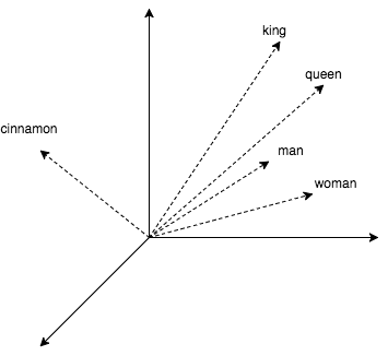
To dilute theory with practice, the article will contain some code where we look for the nearest neighbors for words. Get their vector representations using the popular word2vec. This algorithm produces close vectors for semantically similar words. In word2vec CBOW, vector representations are obtained as a by-product of learning a small neural network that predicts a word from its surroundings. It is curious that with vectors it is possible to turn arithmetic operations like king + (woman - man) = queen.
Let's see how to work with this in the code.
model = gensim.models.KeyedVectors.load_word2vec_format('./GoogleNews-vectors-negative300.bin', binary=True) start = time.time() pprint.pprint(model.wv.most_similar(positive=['king'])) print('time:', time.time() - start) print('king + (woman - man) = ', model.wv.most_similar(positive=['woman', 'king'], negative=['man'])[0]) print('Japan + (Moscow - Russia) = ', model.wv.most_similar(positive=['Moscow', 'Japan'], negative=['Russia'])[0]) We get:
[(u'kings', 0.7138045430183411), (u'queen', 0.6510956883430481), (u'monarch', 0.6413194537162781), (u'crown_prince', 0.6204219460487366), (u'prince', 0.6159993410110474), (u'sultan', 0.5864823460578918), (u'ruler', 0.5797567367553711), (u'princes', 0.5646552443504333), (u'Prince_Paras', 0.5432944297790527), (u'throne', 0.5422105193138123)] time: 0.236690998077 king + (woman - man) = (u'queen', 0.7118192911148071) Japan + (Moscow - Russia) = (u'Tokyo', 0.8696038722991943) In the example above, a library was used to work with the text gensim and word2vec model (1.5 GB) from Google, which has 3 million words and short phrases. The code output shows that queens, monarchs and princes are close to the king. We also made sure that arithmetic with vectors works. However, a quarter of a second per request is not very attractive, and in fact, in gensim, a relatively good implementation of bruteforce search (with calculation of distances to all known objects). Next, we will look at methods that can reduce this time hundreds of times with only a small loss in accuracy.
But let's start with a simple idea: let's try to narrow the search space by dividing it into two halves with a plane. And during the search, we will consider distances only to those neighbors who were on the same side of the plane as the query.
nbrs = NearestNeighbors(algorithm='brute', metric='cosine') nbrs.fit(model.wv.syn0norm) king_vec = model.wv['king'][np.newaxis, :] # start = time.time() idxs = nbrs.kneighbors(king_vec, return_distance=False, n_neighbors=10)[0] print('full search time:', time.time() - start) print([model.wv.index2word[idx] for idx in idxs]) # 2 vec1_idx = random.randint(0, model.wv.syn0norm.shape[0]) vec2_idx = random.randint(0, model.wv.syn0norm.shape[0]) plane = model.wv.syn0norm[vec1_idx] - model.wv.syn0norm[vec2_idx] # -, . # scalar = model.wv.syn0norm.dot(np.transpose(plane)) # if king_vec.dot(plane) > 0: mask = scalar > 0 else: mask = scalar < 0 print('elements in mask:', mask.sum()) half_nbrs = NearestNeighbors(algorithm='brute', metric='cosine') half_nbrs.fit(model.wv.syn0norm[mask]) half_index2word = list(compress(model.wv.index2word, mask)) start = time.time() idxs = half_nbrs.kneighbors(king_vec, return_distance=False, n_neighbors=10)[0] print('half search time:', time.time() - start) print([half_index2word[idx] for idx in idxs]) We get:
full search time: 20.3163180351 [u'king', u'kings', u'queen', u'monarch', u'crown_prince', u'prince', u'sultan', u'ruler', u'princes', u'Prince_Paras'] elements in mask: 1961204 half search time: 9.15824007988 [u'king', u'kings', u'queen', u'monarch', u'crown_prince', u'prince', u'sultan', u'ruler', u'princes', u'Prince_Paras'] So we reduced the computation by half, losing only accuracy next to the plane. Some of the algorithms that we look at next use similar tricks.

1. HNSW
In 2011, one of the best search algorithms for the nearest neighbors of Navigable Small World (NSW) was published. In 2016, his successor Hierarchical Navigable Small World (HNSW) appeared.
Let's start with the parent NSW algorithm. It is based on the “small world” column. These graphs have a curious and useful feature for us: a pair of vertices is not likely to be adjacent, but they can be achieved in a relatively small number of steps ( average). Such graphs are quite common. For example, the brain's neural networks, groups in social networks and the WordNet semantic network are SW columns. In our case, the vertices are vectors, and the edges connect them with the nearest. The graph also presents edges connecting the vertices at a great distance.
To search for neighbors, we go around the graph in search of vertices with the minimum distance to the query. We start from a random vertex, count the distance from the unvisited vertices of the "friends" (vertices connected to the current edge) to the query, and go to the vertex with the smallest distance. Long edges give the graph properties of the close world and allow you to quickly move to the area close to the request objects, and short - eagerly search for the nearest neighbors.

As we go round the graph, we update a small list of our nearest neighbors and stop if the list has not been updated at the next iteration.
K-NNSearch(object q, integer: m, k) 1 TreeSet [object] tempRes, candidates, visitedSet, result 2 for (i←0; i < m; i++) do: 3 put random entry point in candidates 4 tempRes←null 5 repeat: 6 get element c closest from candidates to q 7 remove c from candidates 8 //check stop condition: 9 if c is further than k-th element from result 10 than break repeat 11 //update list of candidates: 12 for every element e from friends of c do: 13 if e is not in visitedSet than 14 add e to visitedSet, candidates, tempRes 15 16 end repeat 17 //aggregate the results: 18 add objects from tempRes to result 19 end for 20 return best k elements from result index = nmslib.init(space='cosinesimil', method='sw-graph') nmslib.addDataPointBatch(index, np.arange(model.wv.syn0.shape[0], dtype=np.int32), model.wv.syn0) index.createIndex({}, print_progress=True) start = time.time() items = nmslib.knnQuery(index, 10, king_vec.tolist()) print(time.time() - start) print([model.wv.index2word[idx] for idx in items]) We get:
0.000545024871826 [u'king', u'kings', u'queen', u'monarch', u'crown_prince', u'prince', u'sultan', u'ruler', u'princes', u'royal'] Consider the development of the idea described above in the Hierarchical Navigable Small World (HNSW) algorithm. It is in many ways similar to NSW, but now we are dealing with a hierarchy of graphs: on the zero layer all objects are represented, and as the layer increases, their subsampling is less and less. In this case, all the objects on the layer there is on the layer .

When searching, a start occurs from a random vertex in the graph of the upper layer; there we quickly find vertices (candidates) close to the query and resume searching from them on the previous layer.
SearchAtLayer (object q, Set[object] enterPoints, integer: M, ef, layer) 1 Set [object] visitedSet 2 priority_queue [object] candidates (closer - first), result (further - first) 3 candidates, visitedSet, result ← enterPoints 7 4 repeat: 5 object c =candidates.top() 6 candidates.pop() 7 //check stop condition: 8 if d(c,q)>d(result.top(),q) do: 9 break 10 //update list of candidates: 11 for_each object e from c.friends(layer) do: 12 if e is not in visitedSet do: 13 add e to visitedSet 14 if d(e, q)< d(result.top(),q) or result.size()<ef do: 15 add e to candidates, result 16 if result.size()>ef do: 17 result.pop() 18 return best k elements from result K-NNSearch (object query, integer: ef) 1 Set [object] tempRes, enterPoints=[enterpoint] 2 for i=maxLayer downto 1 do: 3 tempRes=SearchAtLayer (query, enterPoints, M, 1, i) 4 enterPoints =closest elements from tempRes 5 tempRes=SearchAtLayer (query, enterPoints, M, ef, 0) 6 return best K of tempRes 1.1. Pros & Cons
+ Algorithm is easy to understand.
+ It shows state-of-the-art results.
+ There is an effective implementation in the nmslib library.
+ Small additional memory costs for storing graph edges
- The algorithm does not support the compression of vector representations, which we consider below
index = nmslib.init(space='cosinesimil', method='hnsw') nmslib.addDataPointBatch(index, np.arange(model.wv.syn0.shape[0], dtype=np.int32), model.wv.syn0) index.createIndex({}, print_progress=True) start = time.time() items = nmslib.knnQuery(index, 10, king_vec.tolist()) print(time.time() - start) print([model.wv.index2word[idx] for idx in items]) We get:
0.000469923019409 [u'king', u'kings', u'queen', u'monarch', u'crown_prince', u'prince', u'sultan', u'ruler', u'princes', u'Prince_Paras'] 2. FAISS
In March 2017, Facebook presented its solution for ANN - the FAISS library. It combines many methods and algorithms. In the algorithm, which we consider below, the distances to the groups of vectors will be approached by the distance to the reference point next to them. So we can find out the distance from the request to a small number of reference points, and then brute-force to calculate the distance to the vectors belonging to the reference point, which is the closest to the request. Let us analyze this algorithm in parts.
2.1. ADC - asymmetric distance computation
Let us consider the following idea in more detail: distances to groups of vectors can be approximated by distances to reference points near them. Anchor points divide space into areas. FAISS uses the well-known k-means clustering algorithm to search for control points, and the resulting centroids are mapped to vectors.
 (0.1, 0.2) → 1
 (0.5, -0.2) → 2
 (0.1, 0.1) → 1
 (0.6, -0.1) → 2
Collection vectors are approximated by their centroids. where and - A lot of centroids. Then the distance from the query before can be approached . This method of calculating the distance is called asymmetric. In simple words: we divided the space into regions and said that the distance from the query to a group of vectors falling into one region is approximately equal to the distance to the centroid that forms this region.

Efficiently store and quickly get vectors belonging to the centroid, helps a simple trick called inverted file.
2.2. IVF - inverted file
In IVF, we invert the assignment. Now centroids are matched with lists of vectors.
 1 → [(0.1, 0.2), (0.1, 0.1)]
 2 → [(0.5, -0.2), (0.6, -0.1)]
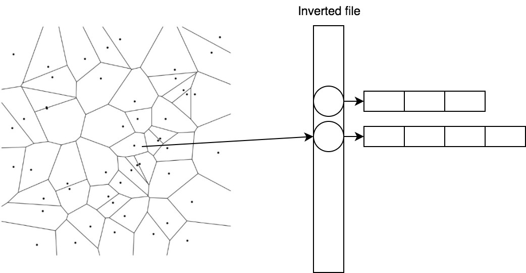
So we can quickly find candidates, considering the distance to the centroids, and then take a ready list for the nearest one.
2.3. PQ - product quantizer
The last component that we touch on in the article is called the product quantizer. It provides lossy vector compression and is used when vector representations do not fit into memory. Suppose that our vectors have a dimension of 128 and we want to encode them with 64 bits (only 0.5 bits per component), then we will have to do quantization with the number of centroids equal to . This is not a trivial task. which also requires a huge training set.
Simplify the task by breaking the vector into parts , and by tradition we find 256 centroids for each of the parts. That is, the vector can be rewritten as a set of centroid indices — for example, , and occupies this economy byte.
This kind of coding will be applied to residual vectors , , and then
2.4. Search
And now we will collect all this in one scheme.

For request we find nearest centroids, collect lists of vectors corresponding to these centroids, and calculate distances to them using residual vectors, and then choose closest.
import faiss index = faiss.index_factory(model.wv.syn0norm.shape[1], 'IVF16384,Flat') index.verbose = True train = model.wv.syn0norm[np.random.binomial(1, 1./3, size=model.wv.syn0norm.shape[0]).astype(bool)] index.train(train) index.add(model.wv.syn0norm) index.nprobe = 100 start = time.time() distances, items = index.search(king_vec, 10) print(time.time() - start) print([model.wv.index2word[idx] for idx in items[0]]) We get:
0.0048999786377 [u'king', u'kings', u'queen', u'monarch', u'crown_prince', u'prince', u'sultan', u'ruler', u'princes', u'Prince_Paras'] 2.5. Pros & Cons
+ Compression support
+ Low storage overhead
+ GPU Calculation Capability *
- Five times slower than HNSW on CPU
* We could not quickly start a GPU implementation out of the box and decided not to waste time on it.
3. ANNOY
The idea of dividing space by planes is well implemented in Annoy . The algorithm is beautifully described by the author in the blog , I recommend to read, if you want to understand the details. I will try to summarize the essence. In the algorithm, we recursively divide the space by planes, forming a binary tree. In each node of the tree is stored the vector that defines the current plane. When searching, we start from the root and select a child node based on the position of the query relative to the plane. So we go down to the leafy elements of the tree, in which the vectors that are on the same side of a group of planes are stored (this is a small piece of space), they are very likely to be the desired nearest neighbors. Let's look at the advantages and disadvantages of Annoy compared to other algorithms.
3.1. Pros & Cons
+ Algorithm is easy to understand.
- It requires a lot of memory
- Loses in speed
4. Comparison of algorithms
Each of the algorithms has a set of parameters, whether it is the maximum number of friends for a vertex (in NSW, HNSW) or the number of centroids (in FAISS). These parameters affect the amount of memory consumed, the quality and speed of the search. The author Annoy implemented tests for a group of ANN algorithms in the ann-benchmarks repository on various parameters. They estimate the accuracy of the search for the ten nearest neighbors in datasets obtained using the GloVe and SIFT algorithms.
GloVe is another way to get vector representations of words, it surpasses word2vec in all indicators when training on a body of the same size. Dataset is composed of 1.2 million vector word representations, trained on 2 billion tweets. SIFT is an old algorithm for obtaining key points of an image and their vector representations that are resistant to transformations. It was used for object recognition, and an important part of this recognition was the search for similar vector representations. There are several variations of datasets, we are interested in SIFT 1M, containing a million vectors.
Below are graphs reflecting the relationship between the speed of the algorithms and the accuracy of the search for the ten nearest neighbors. Algorithms are represented by groups of points, each of the points is the start of a test on a set of parameters.
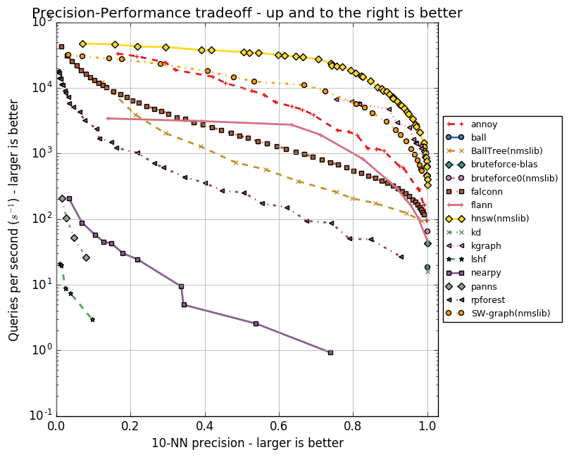
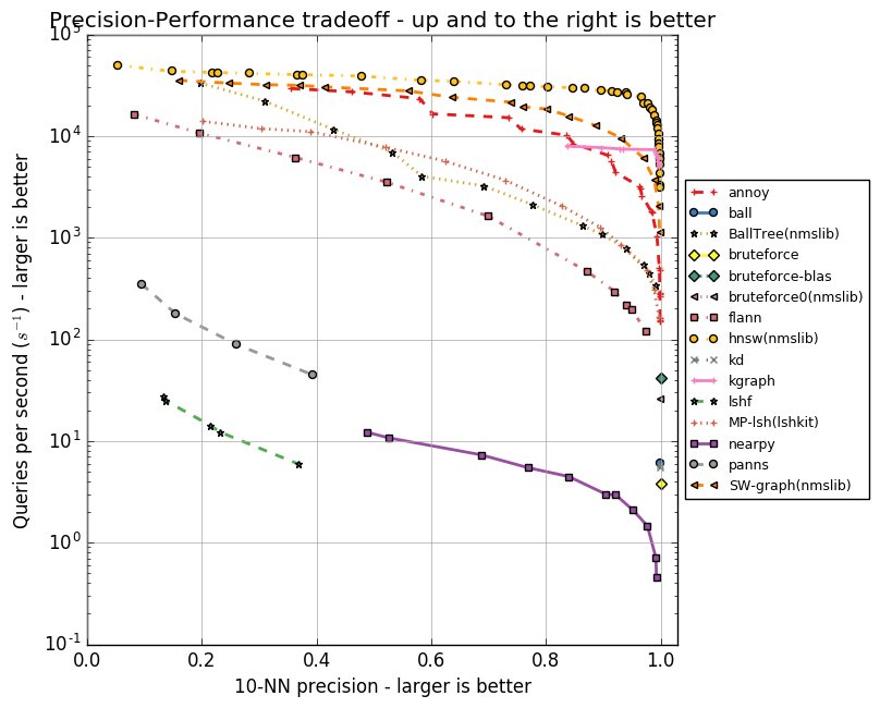
It is clear that HNSW is confidently leading. However, there are no FAISS on the charts. Facebook independently compared HNSW and FAISS in different configurations, the results are shown in the table.
| Method | search time | 1-r @ 1 | index size | index build time |
|---|---|---|---|---|
| Flat-cpu | 9.100 s | 1.0000 | 512 MB | 0 s |
| nmslib (hnsw) | 0.081 s | 0.8195 | 512 + 796 MB | 173 s |
| IVF16384, Flat | 0.538 s | 0.8980 | 512 + 8 MB | 240 s |
| IVF16384, Flat (Titan X) | 0.059 s | 0.8145 | 512 + 8 MB | 5 s |
| Flat-GPU (Titan X) | 0.753 s | 0.9935 | 512 MB | 0 s |
In the table, the FAISS methods are uncompressed, in particular IVF16384,Flat . This means that IVFADC is used with 16,384 centroids. Memory costs are indicated for the case with a million vectors of dimension 128 in float32. HNSW is five times faster in computing on a CPU, but deposited on the edges of a graph ( ) more memory required than centroids ( ).
5. Conclusion
We considered a number of algorithms used to quickly find the nearest neighbors. Annoy lost both by memory and by speed, but the idea is good and can help in solving related problems. For example, the isolation forest anomalies search algorithm, which is convenient for cleaning, is very similar in its idea. FAISS is an excellent solution with memory limitations, it is quite possible to fit a billion vector representations into 60 GB of RAM with it, using IVF16384, PQ64. However, if the memory is not a bottleneck, then you should choose HNSW.
PS The most interesting were publications about algorithms in FAISS. There, for example, you can read about optimizing for the GPU, about the improved quantization method (Optimized Product Quantization) and about a more clever way to build an index (inverted multi-index).
PPS For ourselves, we have chosen HNSW.
6. Literature
- Approximate Nearest Neighbor Search Small World Approach
- Algorithm based on navigable small world graphs
- Hierarchical Navigable Small World graphs
- Product quantization for nearest neighbor search
- SEARCHING IN ONE BILLION VECTORS: RE-RANK WITH SOURCE CODING
- GloVe: Global Vectors for Word Representation
- Object Recognition from Local Scale-Invariant Features
- Isolation forest
- Billion-scale similarity search with GPUs
- Optimized Product Quantization
- The inverted multi-index
')
Source: https://habr.com/ru/post/338360/
All Articles