Data geometry 1. Simplexes and graphs
The starry sky reminds, points are the fundamental abstraction, the basis of the surrounding space.
This is the first article in the series devoted to describing the properties of bases of spaces based on elements (and not vectors). The basis defines the coordinate system - the description of the elements of space in the form of a set of numbers characterizing the position of the element relative to the basis.
If the space is metric, then the basis sets the metric tensors , allowing to determine the distance between the elements of space according to their coordinates.
The basis metric can be set either through the values of scalar products, or through the values of relations between the elements of the basis. Therefore, the basis can be defined both in the usual geometric space and in the dual space of the graph . In geometric space, the elements of the basis are the vertices of the simplex . In the graph - the nodes of the graph.
')
In the first article we will demonstrate the reciprocity of the simplex and the graph. We define the reciprocal metric tensors — the Gramian and the Laplacian of the basis. We associate them with the parameters of graphs and simplexes. Let us show the role of the space normal .
In the second, we define a coordinate system based on a point basis. Two types of mutual coordinates characterize the object - bi- and di-coordinates. In the full basis, the coordinates allow determining the distances between elements outside the basic space.
In the third article, we deal with a useful concept — the scalar product of ordered pairs, which is a generalization of the norm of a vector — the square of the distance between the elements of space.
Next, we turn to the space of the graph. Solve the Dirichlet problem. We show how the concept of the fundamental matrix is connected with the definition of distances between elements outside the space of a subgraph.
In the 5th part, we consider the coordinate transformation when the basis changes. Transformations of point bases are used, for example, in the tasks of localizing sensors (determining their coordinates).
Finally, in conclusion, we consider the basis of the simplest structure, the graph-star. We use it to describe the space of positive integers that are decomposed into a product of simple ones .
Go!
Suppose we have a set consisting of n elements. The elements can be a geometric point in space, a graph node, a letter, a word, a document, a person, etc. — almost any object. Assume that the degree of closeness of the elements of a set is known. For points in space, the degree of proximity is the square of the distance between them. In physics, the measure of closeness between two events is called the interval .
Sometimes, instead of square distance, the term “quadrant” is used , but since it is rarely used, we will more often use the more harmonious term “distance” . Square distance between elements A and B will be denoted as: q ( A , B ) e q u i v q A B . If we are talking about the distances between the elements of a set, the scalar turns into a matrix: Q a b , lowercase indices denote the set. The tuple of distances from a given element of the set to the rest consists of a set of scalar distances:
q P a = [ q P A , q P B , . . . ] q u a d ( 1.1 )
A set of independent points with known distances between them defines a simplex . In two-dimensional space, the simplex is defined by 3 vertices (triangle), in three-dimensional space - 4 (tetrahedron), etc. - the dimension of the simplex is 1 less than the number of its vertices. Vertices are independent if the volume of the simplex is nonzero.
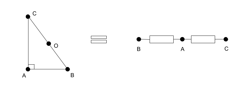
The distances between the vertices of the simplex set the distance matrix Q . The figure shows a right triangle (2-dimensional simplex) with legs 3, 4 and hypotenuse 5. Its distance matrix has the form:
\ begin {array} {c | c c c} Q & A & B & C \\ hline A & 0 & 9 & 16 \\ B & 9 & 0 & 25 \\ C & 16 & 25 & 0 \\ end {array}\ begin {array} {c | c c c} Q & A & B & C \\ hline A & 0 & 9 & 16 \\ B & 9 & 0 & 25 \\ C & 16 & 25 & 0 \\ \ end {array}
For an electrical resistance circuit , the distance is equal to the effective resistance between the nodes of the network. And since any power grid is a graph, in the graph theory, the distance matrix is called the resistance distance matrix . So, the concept of distance is universal - it can be used both for the usual geometric space and for the space of a graph. It also means that a certain graph corresponds to each non-degenerate simplex and vice versa.
At the vertices of a simplex (or graph), one can determine the basis of the space. But to set the metric, you need to define the metric tensor. The distance matrix is not suitable for the role of the metric tensor, if only because its determinant is not related to the volume of the simplex (in the example, to the area of the triangle).
However, as early as the 19th century, A.Cayley (Cayley) discovered that if a distance matrix was edged with a tuple of ones, then the determinant of the resulting matrix would be proportional to the square of the volume of the simplex. The distance -bordered distance matrix is called the Cayley-Menger matrix .
Define the edging operation E d g e symmetric matrices M tuple m a t h b f v and scalar c :
Edge (M, \ mathbf {v}, c) = \ begin {pmatrix} c & v_j \\ v_i & M \\ \ end {pmatrix} \ quad (1.2)Edge (M, \ mathbf {v}, c) = \ begin {pmatrix} c & v_j \\ v_i & M \\ \ end {pmatrix} \ quad (1.2)
If matrix A=Edge(B,..) is bordering the matrix B then B is a submatrix A and is called the main (angular) minor A .
Mathematicians (JCGower) also noticed that it is more convenient to operate not with the distances themselves between the elements, but with negative half-distances −qAB/2 .
This is explained by the fact that negative half-distances reflect the scalar product of elements, as follows from the disclosure of the formula for the square of the distance (distance) between the elements:
q(A,B)=(A−B)2=A2−2A cdotB+B2
From here we get the connection of the distance matrix Q and matrix of scalar products G :
G=( mathbfn mathbf1+ mathbf1 mathbfn−Q)/2 quad(1.3)
Here mathbfn=diag(G) - the norms of the elements, the diagonal of the matrix of scalar products. In the tensor form:
Gij=(ni1j+1inj−Qij)/2
Equally important is the inverse formula - it allows you to get a distance matrix based on Grammians:
Qij=diag(G)i1j+1idiag(G)j−2Gij quad(1.3.1)
Add to the set of ordinary elements of space unusual. Namely - the space normal vector mathbfz . The space of a normal is an orthogonal complement to the space of elements. The scalar product of a normal with elements of the usual space is equal to one, and with itself - zero.
mathbfz cdotA=1, quad mathbfz cdot mathbfz=0 quad(1.4)
The normal is orthogonal to all the vectors of space, therefore it is also called the annihilator . A set of elements containing a space normal will be called major (complete) to distinguish it from a set in which there is no normal. Normal will be put in the set in the first place.
Now we are ready to define the metric tensor. Remote metric tensor Gm is a set of scalar products between elements of a major set:
Gm = Edge (G, \ mathbf {1}, 0) = \ begin {pmatrix} 0 & 1_j \\ 1_i & G_ {ij} \\ \ end {pmatrix} \ quad (1.5)
Matrices of scalar products (vectors) are called Gram matrices . We will use the same term for scalar products of elements, in an abbreviated form - Gramian. Thus, the distance metric tensor is the Gramian of the major basis.
For our simplex of three vertices (right triangle), the distance metric tensor will look like:
\ begin {array} {c | cccc} Gm & * & A & B & C \\ hline * & 0 & 1 & 1 & 1 \\ A & 1 & 0 & -4.5 & -8 \\ B & 1 & -4.5 & 0 & -12.5 \\ C & 1 & -8 & -12.5 & 0 \\ \ end {array}
Note that the dimension of the distance tensor is two more than the dimension of the ordinary vector tensor when describing the space of the same dimension. That is, this tensor contains more information.
For the Gramians we will use the lower indices:
Gmij equivGm
The determinant of the metric tensor Gm associated with the volume of the simplex vol . The exact formula:
(m! vol)2=−det(Gm) quad(1.6)
Where m=l−1 - dimension of the space given by simplex from l vertices.
Calculate the area of our triangle. We have m=2,det(Gm(A,B,C))=−144 . Then 2 vol= sqrt144=12 from where vol=6 . Of course, this area could be obtained by simply multiplying the lengths of the legs. vol=3 cdot4/2 .
Another useful characteristic contained in DMT is the value of the square of the radius of the described sphere around the vertices of the simplex. This m -dimensional sphere plays an important role in the basis, we will call it the basis sphere and denoted as Z . The basic sphere is simply an element of space. Square of its radius rs - this is the norm of this element. The norm of the sphere of a basis is equal to the ratio of the determinants of the angular minor and major Gramians of the basis:
rs=n(Z)=det(G)/det(Gm) quad(1.7)
In our triangle the norm of the sphere will be equal to: rs=−900/−144=$6.2 .
For the metric tensor, there is always an inverse, which is also called reciprocal. The circulation of a remote metric tensor is called the Laplace metric tensor. Lm - LMT. Connection of tensors:
Lm cdotGm=I quad(1.8) where I - unit matrix.
Why did the inverse distance metric tensor become Laplace ? Because its main angular minor (submatrix) is the Laplacian L . The same matrix, which describes the nodes and links in the graph, it is also called the Kirchhoff matrix . We can say that formula (1.8) connects the properties of simplices and graphs. Each Laplacian corresponds to a Gramian and vice versa. Such reciprocity allows us to compare the geometric characteristics of simplexes with the parameters of graphs .
Laplace metric tensor is denoted by superscripts: Lm equivLmij .
The Laplace metric tensor is the major Laplacian, bordered by the ordinary (minor) Laplacian. Edging reflects the parameters of the base sphere (1.7):
Lm = Edge (L, \ mathbf {s}, rs) = \ begin {pmatrix} rs & s ^ j \\ s ^ i & L ^ {ij} \\ \ end {pmatrix} \ quad (1.9)
Scalar rs - this is the norm of the basic sphere (in terms of a graph, its inverse connection), si=b(Z) - barycentric coordinates of the base sphere. Barycentric coordinates are the weight coordinates of an element relative to the base (benchmarks) - the vertices of a simplex or graph. The sum of the weights is equal to one — the normalization condition for the barycentric components.
Revealing the multiplication of metric tensors (1.8) according to the rules of the product of block matrices,
\ begin {pmatrix} 0 & 1_j \\ 1_i & G_ {ij} \ end {pmatrix} \ cdot \ begin {pmatrix} rs & s ^ k \\ s ^ j & L ^ {jk} \ end {pmatrix} = \ begin {pmatrix} 1_j s ^ j & 1_j L ^ {jk} \\ 1_i rs + G_ {ij} s ^ j & 1_i s ^ k + G_ {ij} L ^ {jk} \ end {pmatrix} = \ begin {pmatrix} 1 & 0 ^ k \\ 0_i & I_ {i} ^ {k} \ end {pmatrix} \ quad (1.10)
we get the 4th basic identities.
The sum of the components of the barycentric coordinates of the center of the sphere is 1:
1jsj=1 quad(1.10.1)
The sum of the values of the rows (and columns) of the Laplacian is 0. This means that the rows of the Laplacian are the barycentric coordinates of some vectors:
1jLjk=0k quad(1.10.2) :
Property of equidistance of base vertices (simplex or graph) from the center of a sphere:
Gijsj=−1irs
Finally, the connection of the minor Gramian and Laplacian:
GijLjk=Iki−1isk quad(1.10.4)
View Matrices Iki−1isk where s - a certain barycentric vector, called translation matrices. They can be used, for example, to transfer the origin of a certain data set. X to the point defined by the barycentric coordinates s . Matrix data are projectors .
Let us compare the geometrical parameters of the simplex with the characteristics of the Laplacian.
The matrix tree theorem connects the number of the spanning trees of a graph with the determinant of the minor of the Laplacian. In previous articles, this quantity was called the scalar potential of the Laplacian u :
u(L)=det′(L)=−det(Lm)=−det(Gm)−1=(m! vol)−2 quad(1.12)
Here through det′(L) denoted pseudodeterminant , that is, the determinant from the minor of the Laplacian (since the Laplacian itself is a degenerate matrix). m=l−1 - dimensionality of space, one less than the number of elements of the basis.
We see that the smaller the number of spanning trees of the graph (the simpler its structure), the greater the volume of the corresponding simplex.
Laplacian can be considered both as a characteristic of the simplex and as parameters of connections of the nodes of the graph. In terms of graphs, the laplacian values are the magnitude of the connection between the nodes (with the opposite sign), and on the diagonal is the total sum of the connections of the nodes.
The look of the laplacian for our example:
L (A, B, C) = {1 \ over 144} \ begin {pmatrix} 25 & -16 & -9 \\ -16 & 16 & 0 \\ -9 & 0 & 9 \\ \ end {pmatrix}
Here the conductivity (the weight of the connection) between nodes A and B is 16/144, between nodes A and C 9/144, and there is no connection between nodes B and C.
Now we find out the geometric meaning of the elements of the Laplacian. Each vertex of the simplex can be associated with the corresponding opposite face. The opposite is understood to be the face of the simplex, which does not touch a given node. Obviously, in the general case such a face is multidimensional. In our triangle is the side (segment) opposite to the vertex. In the tetrahedron is a triangle. Dropping a perpendicular from the given vertex to the opposite face, we obtain the height of the vertex of the simplex. Vertex height product hi on the square of the opposite face fi gives simplex volume vol multiplied by the dimension of its space m :
hifi=m vol quad(1.13)
The elements of the Laplacian simplex can be expressed in terms of the heights of the vertices. The diagonal elements of the laplacian are inversely proportional to the heights:
Lii=1/h2i quad(1.14.1)
The height of the vertex is the distance to the subspace of the remaining vertices of the base. That is what
the greater the height of the vertices of the simplex, the less compact the simplex. In terms of the graph - the greater the conductivity (connectivity) of the vertices - the more compact the graph.
The off-diagonal elements are proportional to the cosine of the angle between the faces of the simplex cos(i,j) :
Lij=−cos(i,j)/(hihj) quad(1.14.2)
The right angle between the faces of the simplex is equivalent to the absence of a connection between the corresponding nodes in the graph.
From relations (1.12), (1.13) and (1.14.1) we can obtain the geometric meaning of the relation of the Laplacian trace tr(L) to its scalar potential tr(L) . This value is related to the sum of the squares of the squares of the faces of the simplex:
tr(L)/u(L)=(m−1)!2 sumf2i quad(1.13.1)
Here m−1 - dimension of the face.
Norm of the sphere of basis r s is a natural characteristic of the simplex. Accordingly, this parameter should have an interpretation in the invariants of the graph .
The inverse of the sphere is called curvature . The basis curvature is a suitable characteristic of the general connectivity of the graph. We call this connection spherical and denote traditionally as k . Then
k = 1 / r s q u a d ( 1.15 )
The dimension of the spherical connectivity coincides with the dimension of the magnitude of the connection between the nodes. So, if for electrical networks conduction between nodes is measured in siemens, then spherical connectivity will be in siemens.
If the norm of the sphere of a basis characterizes the connectivity of the graph, then the barycentric coordinates of the sphere indicate the relative distance of the nodes of the graph. The distance of a node is inversely proportional to its connectivity. The less connected with the rest of the graph - the greater the value of its remoteness. Therefore, the barycentric coordinates of the center of the sphere→ s will also be called the distance vector.
Calculate the parameters of the graph popular in Wikipedia .
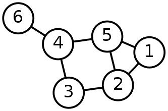
This graph is equivalent to a 6-vertex simplex in 5-dimensional space. Circles with numbers are numbered nodes of the graph. The strength of the connection between the nodes (the value of the weight of the edges) is taken as a unit.
The spherical connectivity of this graph is 1.663 - this is the average connectivity per node. You can compare it with the maximum (7.2) and the minimum (0.8) connection for a graph of 6 nodes. The symmetry index is 0.773.
The distance vector of nodes (barycentric vector of the center of the sphere): [0.364, 0.045, 0.273, -0.227, 0.045, 0.500]. We see that the more a node has connections, the smaller the value of its distance and vice versa. Interestingly the negative value of the distance of the 4th node. This is the only node of the graph, which, when removed, decomposes the graph into two unrelated components. It is possible that the key nodes of the graph have a negative distance.
___
Summing up.The reciprocal metric tensors on the elements of space, the Gramian, and the Laplacian of a major basis are determined. The connection of simplexes and graphs is shown. In the next article we will show how to set the coordinates of the elements in the base.
Table of contents
Introduction
This is the first article in the series devoted to describing the properties of bases of spaces based on elements (and not vectors). The basis defines the coordinate system - the description of the elements of space in the form of a set of numbers characterizing the position of the element relative to the basis.
If the space is metric, then the basis sets the metric tensors , allowing to determine the distance between the elements of space according to their coordinates.
The basis metric can be set either through the values of scalar products, or through the values of relations between the elements of the basis. Therefore, the basis can be defined both in the usual geometric space and in the dual space of the graph . In geometric space, the elements of the basis are the vertices of the simplex . In the graph - the nodes of the graph.
')
The outline and content of the series
In the first article we will demonstrate the reciprocity of the simplex and the graph. We define the reciprocal metric tensors — the Gramian and the Laplacian of the basis. We associate them with the parameters of graphs and simplexes. Let us show the role of the space normal .
In the second, we define a coordinate system based on a point basis. Two types of mutual coordinates characterize the object - bi- and di-coordinates. In the full basis, the coordinates allow determining the distances between elements outside the basic space.
In the third article, we deal with a useful concept — the scalar product of ordered pairs, which is a generalization of the norm of a vector — the square of the distance between the elements of space.
Next, we turn to the space of the graph. Solve the Dirichlet problem. We show how the concept of the fundamental matrix is connected with the definition of distances between elements outside the space of a subgraph.
In the 5th part, we consider the coordinate transformation when the basis changes. Transformations of point bases are used, for example, in the tasks of localizing sensors (determining their coordinates).
Finally, in conclusion, we consider the basis of the simplest structure, the graph-star. We use it to describe the space of positive integers that are decomposed into a product of simple ones .
Go!
Distance matrix
Suppose we have a set consisting of n elements. The elements can be a geometric point in space, a graph node, a letter, a word, a document, a person, etc. — almost any object. Assume that the degree of closeness of the elements of a set is known. For points in space, the degree of proximity is the square of the distance between them. In physics, the measure of closeness between two events is called the interval .
Sometimes, instead of square distance, the term “quadrant” is used , but since it is rarely used, we will more often use the more harmonious term “distance” . Square distance between elements A and B will be denoted as: q ( A , B ) e q u i v q A B . If we are talking about the distances between the elements of a set, the scalar turns into a matrix: Q a b , lowercase indices denote the set. The tuple of distances from a given element of the set to the rest consists of a set of scalar distances:
q P a = [ q P A , q P B , . . . ] q u a d ( 1.1 )
A set of independent points with known distances between them defines a simplex . In two-dimensional space, the simplex is defined by 3 vertices (triangle), in three-dimensional space - 4 (tetrahedron), etc. - the dimension of the simplex is 1 less than the number of its vertices. Vertices are independent if the volume of the simplex is nonzero.
The distances between the vertices of the simplex set the distance matrix Q . The figure shows a right triangle (2-dimensional simplex) with legs 3, 4 and hypotenuse 5. Its distance matrix has the form:
\ begin {array} {c | c c c} Q & A & B & C \\ hline A & 0 & 9 & 16 \\ B & 9 & 0 & 25 \\ C & 16 & 25 & 0 \\ end {array}\ begin {array} {c | c c c} Q & A & B & C \\ hline A & 0 & 9 & 16 \\ B & 9 & 0 & 25 \\ C & 16 & 25 & 0 \\ \ end {array}
For an electrical resistance circuit , the distance is equal to the effective resistance between the nodes of the network. And since any power grid is a graph, in the graph theory, the distance matrix is called the resistance distance matrix . So, the concept of distance is universal - it can be used both for the usual geometric space and for the space of a graph. It also means that a certain graph corresponds to each non-degenerate simplex and vice versa.
Matrix Edging
At the vertices of a simplex (or graph), one can determine the basis of the space. But to set the metric, you need to define the metric tensor. The distance matrix is not suitable for the role of the metric tensor, if only because its determinant is not related to the volume of the simplex (in the example, to the area of the triangle).
However, as early as the 19th century, A.Cayley (Cayley) discovered that if a distance matrix was edged with a tuple of ones, then the determinant of the resulting matrix would be proportional to the square of the volume of the simplex. The distance -bordered distance matrix is called the Cayley-Menger matrix .
Define the edging operation E d g e symmetric matrices M tuple m a t h b f v and scalar c :
Edge (M, \ mathbf {v}, c) = \ begin {pmatrix} c & v_j \\ v_i & M \\ \ end {pmatrix} \ quad (1.2)Edge (M, \ mathbf {v}, c) = \ begin {pmatrix} c & v_j \\ v_i & M \\ \ end {pmatrix} \ quad (1.2)
If matrix A=Edge(B,..) is bordering the matrix B then B is a submatrix A and is called the main (angular) minor A .
About using indexes
The upper and / or lower position of the indices next to the tensor determines the type of tensor. If rank 1 tensors differ only by the position of the indices ( vi and vj , for example), they form a mutual pair.
According to the rules of the product of tensors, the scalar product (convolution, the result is a scalar) are two identical indices at different heights ( aibi ), the dot product (the result is a tuple) - the same indices at the same height ( aibi or aibi ), the outer work (the result is a matrix, a dyad) is two different indices ( aibj or aibj ).
Capital letter in the measurement index means that we are talking about a fixed value in this dimension - the element ( vA - tuple value v element A ).
Where the nature of the object is clear from the context, the indices in the notation will be omitted.
Remote metric tensor (DMT) - basis grammian
Mathematicians (JCGower) also noticed that it is more convenient to operate not with the distances themselves between the elements, but with negative half-distances −qAB/2 .
This is explained by the fact that negative half-distances reflect the scalar product of elements, as follows from the disclosure of the formula for the square of the distance (distance) between the elements:
q(A,B)=(A−B)2=A2−2A cdotB+B2
From here we get the connection of the distance matrix Q and matrix of scalar products G :
G=( mathbfn mathbf1+ mathbf1 mathbfn−Q)/2 quad(1.3)
Here mathbfn=diag(G) - the norms of the elements, the diagonal of the matrix of scalar products. In the tensor form:
Gij=(ni1j+1inj−Qij)/2
Equally important is the inverse formula - it allows you to get a distance matrix based on Grammians:
Qij=diag(G)i1j+1idiag(G)j−2Gij quad(1.3.1)
Add to the set of ordinary elements of space unusual. Namely - the space normal vector mathbfz . The space of a normal is an orthogonal complement to the space of elements. The scalar product of a normal with elements of the usual space is equal to one, and with itself - zero.
mathbfz cdotA=1, quad mathbfz cdot mathbfz=0 quad(1.4)
The normal is orthogonal to all the vectors of space, therefore it is also called the annihilator . A set of elements containing a space normal will be called major (complete) to distinguish it from a set in which there is no normal. Normal will be put in the set in the first place.
Now we are ready to define the metric tensor. Remote metric tensor Gm is a set of scalar products between elements of a major set:
Gm = Edge (G, \ mathbf {1}, 0) = \ begin {pmatrix} 0 & 1_j \\ 1_i & G_ {ij} \\ \ end {pmatrix} \ quad (1.5)
Matrices of scalar products (vectors) are called Gram matrices . We will use the same term for scalar products of elements, in an abbreviated form - Gramian. Thus, the distance metric tensor is the Gramian of the major basis.
For our simplex of three vertices (right triangle), the distance metric tensor will look like:
\ begin {array} {c | cccc} Gm & * & A & B & C \\ hline * & 0 & 1 & 1 & 1 \\ A & 1 & 0 & -4.5 & -8 \\ B & 1 & -4.5 & 0 & -12.5 \\ C & 1 & -8 & -12.5 & 0 \\ \ end {array}
Note that the dimension of the distance tensor is two more than the dimension of the ordinary vector tensor when describing the space of the same dimension. That is, this tensor contains more information.
For the Gramians we will use the lower indices:
Gmij equivGm
The geometric properties of DMT
The determinant of the metric tensor Gm associated with the volume of the simplex vol . The exact formula:
(m! vol)2=−det(Gm) quad(1.6)
Where m=l−1 - dimension of the space given by simplex from l vertices.
Calculate the area of our triangle. We have m=2,det(Gm(A,B,C))=−144 . Then 2 vol= sqrt144=12 from where vol=6 . Of course, this area could be obtained by simply multiplying the lengths of the legs. vol=3 cdot4/2 .
Another useful characteristic contained in DMT is the value of the square of the radius of the described sphere around the vertices of the simplex. This m -dimensional sphere plays an important role in the basis, we will call it the basis sphere and denoted as Z . The basic sphere is simply an element of space. Square of its radius rs - this is the norm of this element. The norm of the sphere of a basis is equal to the ratio of the determinants of the angular minor and major Gramians of the basis:
rs=n(Z)=det(G)/det(Gm) quad(1.7)
In our triangle the norm of the sphere will be equal to: rs=−900/−144=$6.2 .
Laplace metric tensor (LMT) - the basis Laplacian
For the metric tensor, there is always an inverse, which is also called reciprocal. The circulation of a remote metric tensor is called the Laplace metric tensor. Lm - LMT. Connection of tensors:
Lm cdotGm=I quad(1.8) where I - unit matrix.
Why did the inverse distance metric tensor become Laplace ? Because its main angular minor (submatrix) is the Laplacian L . The same matrix, which describes the nodes and links in the graph, it is also called the Kirchhoff matrix . We can say that formula (1.8) connects the properties of simplices and graphs. Each Laplacian corresponds to a Gramian and vice versa. Such reciprocity allows us to compare the geometric characteristics of simplexes with the parameters of graphs .
Laplace metric tensor is denoted by superscripts: Lm equivLmij .
LMT structure
The Laplace metric tensor is the major Laplacian, bordered by the ordinary (minor) Laplacian. Edging reflects the parameters of the base sphere (1.7):
Lm = Edge (L, \ mathbf {s}, rs) = \ begin {pmatrix} rs & s ^ j \\ s ^ i & L ^ {ij} \\ \ end {pmatrix} \ quad (1.9)
Scalar rs - this is the norm of the basic sphere (in terms of a graph, its inverse connection), si=b(Z) - barycentric coordinates of the base sphere. Barycentric coordinates are the weight coordinates of an element relative to the base (benchmarks) - the vertices of a simplex or graph. The sum of the weights is equal to one — the normalization condition for the barycentric components.
The barycentric coordinates of the circumcircle of a right triangle are always the same.
And equal mathbfs=[sA,sB,sC]=[0,0.5,0.5] .
This means that the center O is balanced by equal masses of the elements B and C.
Generally speaking, for any graph that is a chain of series-connected links, the coordinates of the base sphere will be nonzero only at the extreme nodes and equal to 0.5.
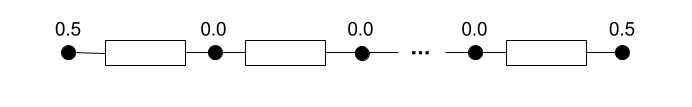
This means that the center O is balanced by equal masses of the elements B and C.
Generally speaking, for any graph that is a chain of series-connected links, the coordinates of the base sphere will be nonzero only at the extreme nodes and equal to 0.5.
Minor identities
Revealing the multiplication of metric tensors (1.8) according to the rules of the product of block matrices,
\ begin {pmatrix} 0 & 1_j \\ 1_i & G_ {ij} \ end {pmatrix} \ cdot \ begin {pmatrix} rs & s ^ k \\ s ^ j & L ^ {jk} \ end {pmatrix} = \ begin {pmatrix} 1_j s ^ j & 1_j L ^ {jk} \\ 1_i rs + G_ {ij} s ^ j & 1_i s ^ k + G_ {ij} L ^ {jk} \ end {pmatrix} = \ begin {pmatrix} 1 & 0 ^ k \\ 0_i & I_ {i} ^ {k} \ end {pmatrix} \ quad (1.10)
we get the 4th basic identities.
The sum of the components of the barycentric coordinates of the center of the sphere is 1:
1jsj=1 quad(1.10.1)
The sum of the values of the rows (and columns) of the Laplacian is 0. This means that the rows of the Laplacian are the barycentric coordinates of some vectors:
1jLjk=0k quad(1.10.2) :
Property of equidistance of base vertices (simplex or graph) from the center of a sphere:
Gijsj=−1irs
Finally, the connection of the minor Gramian and Laplacian:
GijLjk=Iki−1isk quad(1.10.4)
View Matrices Iki−1isk where s - a certain barycentric vector, called translation matrices. They can be used, for example, to transfer the origin of a certain data set. X to the point defined by the barycentric coordinates s . Matrix data are projectors .
Construction of distance matrix for Laplacian
If we are dealing with a graph, then to build a distance matrix based on the adjacency matrix C You can use the following algorithm. For the adjacency matrix, we build the Laplacian:
L=Diag(C cdot mathbf1)−C quad(1.11.1)
Here Diag() - transformation of a tuple into a diagonal matrix.
The determinant of the Laplacian is zero, so it cannot simply be reversed. It is necessary either to remove some node from it, or to supplement (border) with some vector.
We border the Laplacian with a vector of units and reverse the resulting matrix. The main minor (submatrix) of the result of the call will be the Green matrix. Gr .
\ begin {pmatrix} 0 & 1 ^ j \\ 1 ^ i & L ^ {ij} \ end {pmatrix} ^ {- 1} = \ begin {pmatrix} 0 & / l_j \\ / l_i & Gr_ {ij } \ end {pmatrix} \ quad (1.11.2)
l - the number of vertices of the basis.
The Green matrix is a Gramian - a matrix of scalar products of vectors directed from the center of coordinates (here it is a base centroid) to the elements. To obtain the distance matrix from the Gramian one should use the formula (1.3.1).
Let be Gr equiv(A−C) cdot(B−C) where C - Centre. Then the formula (1.3.1) takes the following form:
Q=(A−C)2+(B−C)2−2(A−C) cdot(B−C)=(A−B)2
Laplacian geometry
Let us compare the geometrical parameters of the simplex with the characteristics of the Laplacian.
The volume of the simplex and the potential of the laplacian
The matrix tree theorem connects the number of the spanning trees of a graph with the determinant of the minor of the Laplacian. In previous articles, this quantity was called the scalar potential of the Laplacian u :
u(L)=det′(L)=−det(Lm)=−det(Gm)−1=(m! vol)−2 quad(1.12)
Here through det′(L) denoted pseudodeterminant , that is, the determinant from the minor of the Laplacian (since the Laplacian itself is a degenerate matrix). m=l−1 - dimensionality of space, one less than the number of elements of the basis.
We see that the smaller the number of spanning trees of the graph (the simpler its structure), the greater the volume of the corresponding simplex.
Elements of laplacian
Laplacian can be considered both as a characteristic of the simplex and as parameters of connections of the nodes of the graph. In terms of graphs, the laplacian values are the magnitude of the connection between the nodes (with the opposite sign), and on the diagonal is the total sum of the connections of the nodes.
The look of the laplacian for our example:
L (A, B, C) = {1 \ over 144} \ begin {pmatrix} 25 & -16 & -9 \\ -16 & 16 & 0 \\ -9 & 0 & 9 \\ \ end {pmatrix}
Here the conductivity (the weight of the connection) between nodes A and B is 16/144, between nodes A and C 9/144, and there is no connection between nodes B and C.
Now we find out the geometric meaning of the elements of the Laplacian. Each vertex of the simplex can be associated with the corresponding opposite face. The opposite is understood to be the face of the simplex, which does not touch a given node. Obviously, in the general case such a face is multidimensional. In our triangle is the side (segment) opposite to the vertex. In the tetrahedron is a triangle. Dropping a perpendicular from the given vertex to the opposite face, we obtain the height of the vertex of the simplex. Vertex height product hi on the square of the opposite face fi gives simplex volume vol multiplied by the dimension of its space m :
hifi=m vol quad(1.13)
The elements of the Laplacian simplex can be expressed in terms of the heights of the vertices. The diagonal elements of the laplacian are inversely proportional to the heights:
Lii=1/h2i quad(1.14.1)
The height of the vertex is the distance to the subspace of the remaining vertices of the base. That is what
the greater the height of the vertices of the simplex, the less compact the simplex. In terms of the graph - the greater the conductivity (connectivity) of the vertices - the more compact the graph.
The off-diagonal elements are proportional to the cosine of the angle between the faces of the simplex cos(i,j) :
Lij=−cos(i,j)/(hihj) quad(1.14.2)
The right angle between the faces of the simplex is equivalent to the absence of a connection between the corresponding nodes in the graph.
From relations (1.12), (1.13) and (1.14.1) we can obtain the geometric meaning of the relation of the Laplacian trace tr(L) to its scalar potential tr(L) . This value is related to the sum of the squares of the squares of the faces of the simplex:
tr(L)/u(L)=(m−1)!2 sumf2i quad(1.13.1)
Here m−1 - dimension of the face.
Sphere of basis and graph connectivity
Norm of the sphere of basis r s is a natural characteristic of the simplex. Accordingly, this parameter should have an interpretation in the invariants of the graph .
The inverse of the sphere is called curvature . The basis curvature is a suitable characteristic of the general connectivity of the graph. We call this connection spherical and denote traditionally as k . Then
k = 1 / r s q u a d ( 1.15 )
The dimension of the spherical connectivity coincides with the dimension of the magnitude of the connection between the nodes. So, if for electrical networks conduction between nodes is measured in siemens, then spherical connectivity will be in siemens.
Spherical connected values in various topologies of the graph
For a complete graph (all nodes are connected to all) with the same communication strength c expression for connectivity depending on the number of nodes l has the following form:
kmax(l)=c l2/(l−1) quad(1.16.1)
In large graphs, the value of the connection coincides with the number of links of the node, which is expected from such an invariant.
Formula (1.16.1) expresses the maximum value of connectivity for a given number of nodes. The minimal is the connectivity of trees - graphs without cycles with one connected component. Trees include, for example, an open chain and a star. The expression for minimal connectivity is:
kmin(l)=4c/(l−1) quad(1.16.2)
For comparison, we also give the closed circuit connectivity - an intermediate value between the maximum and minimum connectivity:
kclosed(l)=12 l c/(l2−1) quad(1.16.3)
In both cases, connectivity falls linearly with increasing graph size.
If the norm of the sphere of a basis characterizes the connectivity of the graph, then the barycentric coordinates of the sphere indicate the relative distance of the nodes of the graph. The distance of a node is inversely proportional to its connectivity. The less connected with the rest of the graph - the greater the value of its remoteness. Therefore, the barycentric coordinates of the center of the sphere→ s will also be called the distance vector.
Example of parameter values for a graph
Calculate the parameters of the graph popular in Wikipedia .
This graph is equivalent to a 6-vertex simplex in 5-dimensional space. Circles with numbers are numbered nodes of the graph. The strength of the connection between the nodes (the value of the weight of the edges) is taken as a unit.
The spherical connectivity of this graph is 1.663 - this is the average connectivity per node. You can compare it with the maximum (7.2) and the minimum (0.8) connection for a graph of 6 nodes. The symmetry index is 0.773.
The distance vector of nodes (barycentric vector of the center of the sphere): [0.364, 0.045, 0.273, -0.227, 0.045, 0.500]. We see that the more a node has connections, the smaller the value of its distance and vice versa. Interestingly the negative value of the distance of the 4th node. This is the only node of the graph, which, when removed, decomposes the graph into two unrelated components. It is possible that the key nodes of the graph have a negative distance.
___
Summing up.The reciprocal metric tensors on the elements of space, the Gramian, and the Laplacian of a major basis are determined. The connection of simplexes and graphs is shown. In the next article we will show how to set the coordinates of the elements in the base.
Source: https://habr.com/ru/post/338186/
All Articles