“Use the Power of Machine Learning, Luke!” Or automatic classification of luminaires according to the CIL

“The power of machine learning among us, its methods surround us and bind. The power around me, everywhere, between me, you, the decisive tree, the lasso, the crest and the support vector "

So, probably, Yoda would tell me if he taught me the ways of Data Science.



Unfortunately, so far among my acquaintances, green-skinned wrinkled personalities are not observed, so we simply continue along with you our joint way of teaching data science from the absolute novice level to ... a real Jedi of what we end up with.



In the last two articles, we solved the problem of classifying light sources according to their spectrum (in Python and C #, respectively). This time we will try to solve the problem of classifying luminaires according to their light intensity curve (according to the spot they shine on the floor).

')

If you have already comprehended the path of power, you can immediately download the dataset on Github and play around with this task yourself. But everyone, as I am newbies ask tackle.



Fortunately, the task at this time is quite simple and does not take much time.







I really wanted to start the table of contents sections of the article from the fourth episode, but its name did not fit the meaning.

Episode I: A hidden threat or what threatens you if you have not read the entire previous cycle of articles.

Well, in principle, nothing threatens, but if you are completely new to Data Science, I advise you to still look at the first articles in the correct chronological order, because this is in some way a valuable experience of looking at Data Science through the eyes of a beginner, if I had to describe my path now, then I would not be able to recall those sensations and some of the problems would have seemed to me quite funny. Therefore, if you have just started, look at how I suffered (and still suffer) mastering the very basics and you will understand that you are not so alone and all your problems in mastering machine learning and data analysis are completely solvable.



So, here is a list of articles in order of appearance (from first to last)

• “ Catch data big and small! "- (Overview of Cognitive Class Data Science Courses)
• " Now he counted you " or Data Science from Scratch
• “ Iceberg instead of Oscar! "Or as I tried to learn the basics of DataScience on kaggle
• “ “ A train that could! ”Or“ Specialization Machine learning and data analysis ”, through the eyes of a newbie in Data Science
• “Rise of Machinery Learning” or combine a hobby in Data Science and analyzing the spectra of light bulbs
• “ “ As per the notes! ”Or Machine Learning (Data science) in C # using Accord .NET Framework

Also, at the request of the workers in particular, the user GadPetrovich starting with this article will make a table of contents for the material.



Content:

Episode I: The hidden threat or what threatens you if you have not yet read the entire previous series of articles.

Episode II: Attack of the Clones or it seems that this task is not much different from the previous one.

Episode III: Revenge of the Sith or a little about the difficulties of data mining

Episode IV: A New Hope that Everything Is Easily Classified

Episode V: The Empire Strikes Back or is Difficult in Preparing Data Easily in a “Battle”

Episode VI: Return of the Jedi or feel the power of models that were written in advance for you!

Episode VII: The Force Awakens - Instead of Conclusion

Episode II: Attack of the clones or it seems that this task is not much different from the past.

Hmm, just the second title, and I already think that it will be hard to continue to adhere to the style.



So, let me remind you that last time you and I considered the following issues: creating your own data set for machine learning tasks, training models of classifiers of these data using the example of logistic regression and random forest, as well as visualization and classification using PCA, T-SNE and DBSCAN.

This time the task will not be radically different, though the signs will be smaller.



Looking a little ahead, I’ll say that in order for the task not to look altogether a clone of the past, this time in the example we will meet the SVC classifier, and also we will clearly see that scaling the source data can be very useful.

Episode III: Revenge of the Sith or a little about the difficulties of data mining.

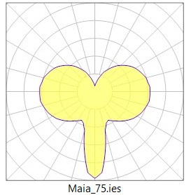
Let's start with what is the light intensity curve (CIL)?

Well, it's about this:





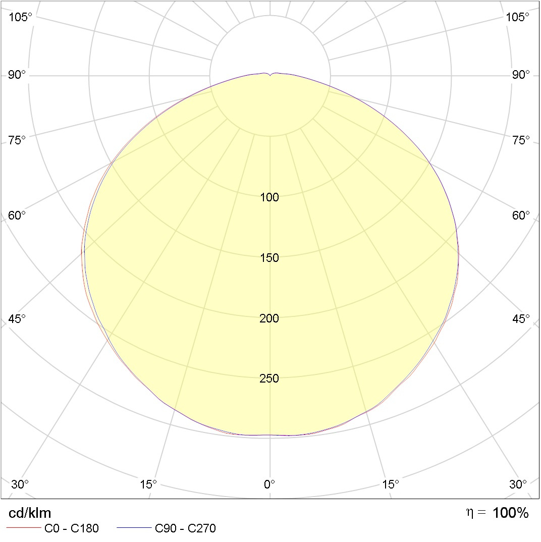
What would have been a little clearer imagine that you have a lamp above your head and just such a cone of light falls under your feet if you stand under it (as in a spot of light from a street lamp).

This picture shows the light intensity (values ​​on the circles) in different polar angles (imagine that this is a longitudinal section of the incandescent lamp), in the gap of two azimuth angles 0-180 and 90 - 270 (imagine that this is a cross section of the incandescent lamp). Maybe I didn’t really, accurately explained, For details on Julian Borisovich Eisenberg in the Lighting Guide p. 833 and on



But back to the original data, do not consider it an advertisement, but all the fixtures that we will classify today will be from one manufacturer, namely, Light Technologies firms. I am not connected with them in any way and my pockets will not be filled with “hard cash” from their mention



Then why are they? It's very simple, the guys have taken care that we were comfortable.

The necessary pictures from the KCC and .ies files for pulling out the data already collected by them in the corresponding archives could only be downloaded , agree that it is much more convenient than to scour the entire network collecting data by grains.



Perhaps an attentive reader, already waiting with impatience to ask where is all this, and why is the section called Sith revenge? Where is the cruel revenge ?!



Well, apparently the revenge of the poems was that for many years I did anything other than math, programming, lighting and machine learning, and now I pay for it with nerve cells.



Let's start a little from afar ...



This is what a simple .ies file looks like.



IESNA:LM-63-1995

[TEST] SL20695

[MANUFAC] PHILIPS

[LUMCAT]

[LUMINAIRE] NA

[LAMP] 3 Step Switch A60 220-240V9.5W-60W 806lm 150D 3000K-6500K Non Dim

[BALLAST] NA

[OTHER] B-Angle = 0.00 B-Tilt = 0.00 2015-12-07

TILT=NONE

1 806.00 1 181 1 1 2 -0.060 -0.060 0.120

1.0 1.0 9.50

0.00 1.00 2.00 3.00 4.00 5.00 6.00 7.00 8.00 9.00

10.00 11.00 12.00 13.00 14.00 15.00 16.00 17.00 18.00 19.00

20.00 21.00 22.00 23.00 24.00 25.00 26.00 27.00 28.00 29.00

30.00 31.00 32.00 33.00 34.00 35.00 36.00 37.00 38.00 39.00

40.00 41.00 42.00 43.00 44.00 45.00 46.00 47.00 48.00 49.00

50.00 51.00 52.00 53.00 54.00 55.00 56.00 57.00 58.00 59.00

60.00 61.00 62.00 63.00 64.00 65.00 66.00 67.00 68.00 69.00

70.00 71.00 72.00 73.00 74.00 75.00 76.00 77.00 78.00 79.00

80.00 81.00 82.00 83.00 84.00 85.00 86.00 87.00 88.00 89.00

90.00 91.00 92.00 93.00 94.00 95.00 96.00 97.00 98.00 99.00

100.00 101.00 102.00 103.00 104.00 105.00 106.00 107.00 108.00 109.00

110.00 111.00 112.00 113.00 114.00 115.00 116.00 117.00 118.00 119.00

120.00 121.00 122.00 123.00 124.00 125.00 126.00 127.00 128.00 129.00

130.00 131.00 132.00 133.00 134.00 135.00 136.00 137.00 138.00 139.00

140.00 141.00 142.00 143.00 144.00 145.00 146.00 147.00 148.00 149.00

150.00 151.00 152.00 153.00 154.00 155.00 156.00 157.00 158.00 159.00

160.00 161.00 162.00 163.00 164.00 165.00 166.00 167.00 168.00 169.00

170.00 171.00 172.00 173.00 174.00 175.00 176.00 177.00 178.00 179.00

180.00

0.00

137.49 137.43 137.41 137.32 137.23 137.10 136.97

136.77 136.54 136.27 136.01 135.70 135.37 135.01

134.64 134.27 133.85 133.37 132.93 132.42 131.93

131.41 130.87 130.27 129.68 129.08 128.44 127.78

127.11 126.40 125.69 124.92 124.18 123.43 122.63

121.78 120.89 120.03 119.20 118.26 117.34 116.40

115.46 114.49 113.53 112.56 111.52 110.46 109.42

108.40 107.29 106.23 105.13 104.03 102.91 101.78

100.64 99.49 98.35 97.15 95.98 94.80 93.65

92.43 91.23 89.99 88.79 87.61 86.42 85.17

83.96 82.76 81.49 80.31 79.13 77.91 76.66

75.46 74.29 73.07 71.87 70.67 69.49 68.33

67.22 66.00 64.89 63.76 62.61 61.46 60.36

59.33 58.19 57.11 56.04 54.98 53.92 52.90

51.84 50.83 49.82 48.81 47.89 46.88 45.92

44.99 44.03 43.11 42.18 41.28 40.39 39.51

38.62 37.74 36.93 36.09 35.25 34.39 33.58

32.79 32.03 31.25 30.46 29.70 28.95 28.23

27.48 26.79 26.11 25.36 24.71 24.06 23.40

22.73 22.08 21.43 20.84 20.26 19.65 19.04

18.45 17.90 17.34 16.83 16.32 15.78 15.28

14.73 14.25 13.71 13.12 12.56 11.94 11.72

11.19 10.51 9.77 8.66 6.96 4.13 0.91

0.20 0.17 0.16 0.19 0.19 0.20 0.16

0.20 0.18 0.20 0.20 0.21 0.20 0.16

0.20 0.17 0.19 0.20 0.19 0.18



Inside, data on the manufacturer and the laboratory of the meter are protected, as well as data on the luminaire directly, including the luminous intensity depending on the polar and azimuth angles, the data about which we need.



In total, I selected 193 files for you, and it is unlikely that I would even try to process them manually.



On the one hand, everything is just a GOST in which the structure of the .ies file is described in detail. On the other hand, it became more difficult to automatically recognize and remove the necessary data than I thought, it cost me a couple of disturbing and sleepless nights.

But for you, as in the best traditions of the cinema, all the complex and tedious things will remain "behind the scenes." Therefore, we proceed to the direct description of the data.

Episode IV: A new hope ... that everything is classified easily and simply.

So, having penetrated into the key issues with the help of the literature to which I referred above, we will come to the conclusion that in order to classify the lamps in our teaching and demonstration example, we have enough of a complete cut of data for any one azimuth angle in this case equal to zero and in the range of polar angles from 0 to 180, with a step of 10 (a step less does not make sense to take on quality, this will not affect much).

That is, in our case, the data will not look like on the graph on the left, but as on the graph on the right.





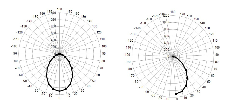
By the way, if anyone did not know, then using the radar chart in MS Excel, you can conveniently construct KCC charts.



Since in the archive of Light Technologies, lamps with different KCCs are unevenly distributed, we will analyze with you 4 types that are most in the original data set.



So, we have the following KCC:

Concentrated (K), deep (G), cosine (D) and semi-wide (L).

Their zones of directions of maximum luminous intensity are in the following corners, respectively:

K = 0 ° -15 °; G = 0 ° -30 °; D = 0 ° -35 °; L = 35 ° -55 °;

Labels for them in the data set are assigned to

K 1; G = 2; D = 3; L = 4; (I had to start from scratch, but now I’m too lazy to redo it)



In fact, not being an expert in the field of lighting, it is difficult to classify lamps, for example, I would attribute the lamp in the figure above to a lamp from a deep CIL, but I am not 100% sure.



In principle, I tried to avoid controversial issues, look at GOST and examples, but I could well be mistaken somewhere, if you find inaccuracies in the assignment of class labels, write, correct as much as possible

Episode V: The Empire Strikes Back or is Difficult in Preparing Data Easily in a “Battle”

Well, it seems that two people can play this game. If it was difficult to prepare the data, then it is just the opposite to analyze. Let's start slowly.

Once again I remind you that the file with all the source code below in .ipynb format (Jupyter) can be downloaded from GitHub



So, to start importing libraries:

 #import libraries import warnings warnings.filterwarnings('ignore') import pandas as pd import numpy as np import matplotlib.pyplot as plt import matplotlib.patches as mpatches from sklearn.model_selection import train_test_split from sklearn . svm import SVC from sklearn.metrics import f1_score from sklearn.ensemble import RandomForestClassifier from scipy.stats import uniform as sp_rand from sklearn.model_selection import StratifiedKFold from sklearn.preprocessing import MinMaxScaler from sklearn.manifold import TSNE from IPython.display import display from sklearn.metrics import accuracy_score from sklearn.model_selection import train_test_split %matplotlib inline    <source lang="python"> #reading data train_df=pd.read_csv('lidc_data\\train.csv',sep='\t',index_col=None) test_df=pd.read_csv('lidc_data\\test.csv',sep='\t',index_col=None) print('train shape {0}, test shape {1}]'. format(train_df.shape, test_df.shape)) display('train:',train_df.head(4),'test:',test_df.head(4)) #divide the data and labels X_train=np.array(train_df.iloc[:,1:-1]) X_test=np.array(test_df.iloc[:,1:-1]) y_train=np.array(train_df['label']) y_test=np.array(test_df['label']) 

If you have read previous articles or are familiar with machine learning in python, then all the code presented here will not be difficult for you.

But just in case, at the beginning we considered the data on training and test samples in the tables, and then we cut out arrays containing signs (luminous intensity in polar angles) and class marks, and of course, for clarity, we printed the first 4 lines from the table , that's what happened:







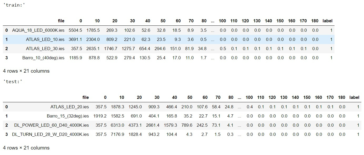
You can take my word for it, the data is less balanced with the exception of class 4 (curve L) and, in general, for the first three classes, we have a ratio of 40 samples in the training sample and 12 in the control, for class L - 28 in the training and 9 in the control as a whole, the ratio close to ¼ between the training and the control sample is preserved.

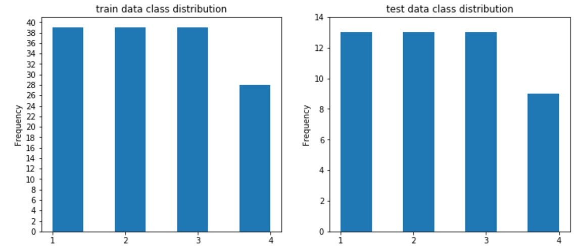
Well, if you are accustomed to not believing anyone, then run the code:

 #draw classdistributions test_n_max=test_df.label.value_counts().max() train_n_max=train_df.label.value_counts().max() fig, axes = plt.subplots(nrows=1, ncols=2, figsize=(12,5)) train_df.label.plot.hist(ax=axes[0],title='train data class distribution', bins=7,yticks=np.arange(0,train_n_max+2,2), xticks=np.unique(train_df.label.values)) test_df.label.plot.hist(ax=axes[1],ti 

And you will see the following:







Let's go back to our signs, as you understand, on the one hand, they all reflect one and the same value, that is, roughly speaking, we do not correlate the number of bicycles and atmospheric pressure, on the other hand, unlike last time , when we had about one sign level of values, this time the amplitude of values ​​can reach tens of thousands of units.



Therefore, it is reasonable to scale the signs. However, all scikit-learn scaling models seem to be scaled by columns (or I didn't figure it out), and it makes no sense for us to scale by columns in this case, it does not equal the “rich” and “poor” lamps, which will lead to class classification tension, so to speak. !



We will instead scale the data by samples (by rows) in order to preserve the character of the distribution of the light intensity over the corners, but at the same time drive the entire spread into the range between 0 and 1.



In a good way, in the books that I read, they give advice on scaling the training sample and the control one model (trained in the training sample), but in our case, this will not happen because of a mismatch in the number of features (in the test sample there are fewer rows and the transposed matrix will have fewer columns), so we equalize each sample in its own way.



Looking ahead to this task, in the process of classification, I did not find anything wrong with that.

 #scaled all data for final prediction scl=MinMaxScaler() X_train_scl=scl.fit_transform(X_train.T).T X_test_scl=scl.fit_transform(X_test.T).T #scaled part of data for test X_train_part, X_test_part, y_train_part, y_test_part = train_test_split(X_train, y_train, test_size=0.20, stratify=y_train, random_state=42) scl=MinMaxScaler() X_train_part_scl=scl.fit_transform(X_train_part.T).T X_test_part_scl=scl.fit_transform(X_test_part.T).T 

Even if you are completely new, during the article you will notice that all models from the scikit-learn set have a similar interface, we train the model by passing the data to the fit method, if we need to transform the data, we call the transform method (in our case we use the 2 in 1), and if it is necessary to predict the data later, we call the method predict and feed it our new (control) samples.



Well, one more small moment, let's imagine that we have no labels for the control sample, for example, we solve the problem on the kagle, how can we then assess the quality of the prediction model?



I think for our case, where the solution of business problems is not required, one of the easiest ways would be to divide the training sample into another training (but smaller) and test (from the training), this will come in handy for us a little later. In the meantime, let's go back to scaling and see how it helped us, the upper picture without scaling features, the bottom one with scaling.

 #not scaled x=np.arange(0,190,10) plt.figure(figsize=(17,10)) plt.plot(x,X_train[13]) plt.plot(x,X_train[109]) plt.plot(x,X_train[68]) plt.plot(x,X_train[127]) c1 = mpatches.Patch( color='blue', label='class 1') c2 = mpatches.Patch( color='green', label='class 2') c3 = mpatches.Patch(color='orange', label='class 3') c4 = mpatches.Patch( color='red',label='class 4') plt.legend(handles=[c1,c2,c3,c4]) plt.xlabel('  (polar angle)') plt.ylabel('  (luminous intensity)') plt.title('   ') 

“Score” it in different cells (well, or make a subplot)

 #scaled x=np.arange(0,190,10) plt.figure(figsize=(17,10)) plt.legend() plt.plot(x,X_train_scl[13],color='blue') plt.plot(x,X_train_scl[109],color='green') plt.plot(x,X_train_scl[68], color='orange') plt.plot(x,X_train_scl[127], color='red') c1 = mpatches.Patch( color='blue', label='class 1') c2 = mpatches.Patch( color='green', label='class 2') c3 = mpatches.Patch(color='orange', label='class 3') c4 = mpatches.Patch( color='red',label='class 4') plt.legend(handles=[c1,c2,c3,c4]) plt.xlabel('  (polar angle)') plt.ylabel('  (luminous intensity)') plt.title('    ()')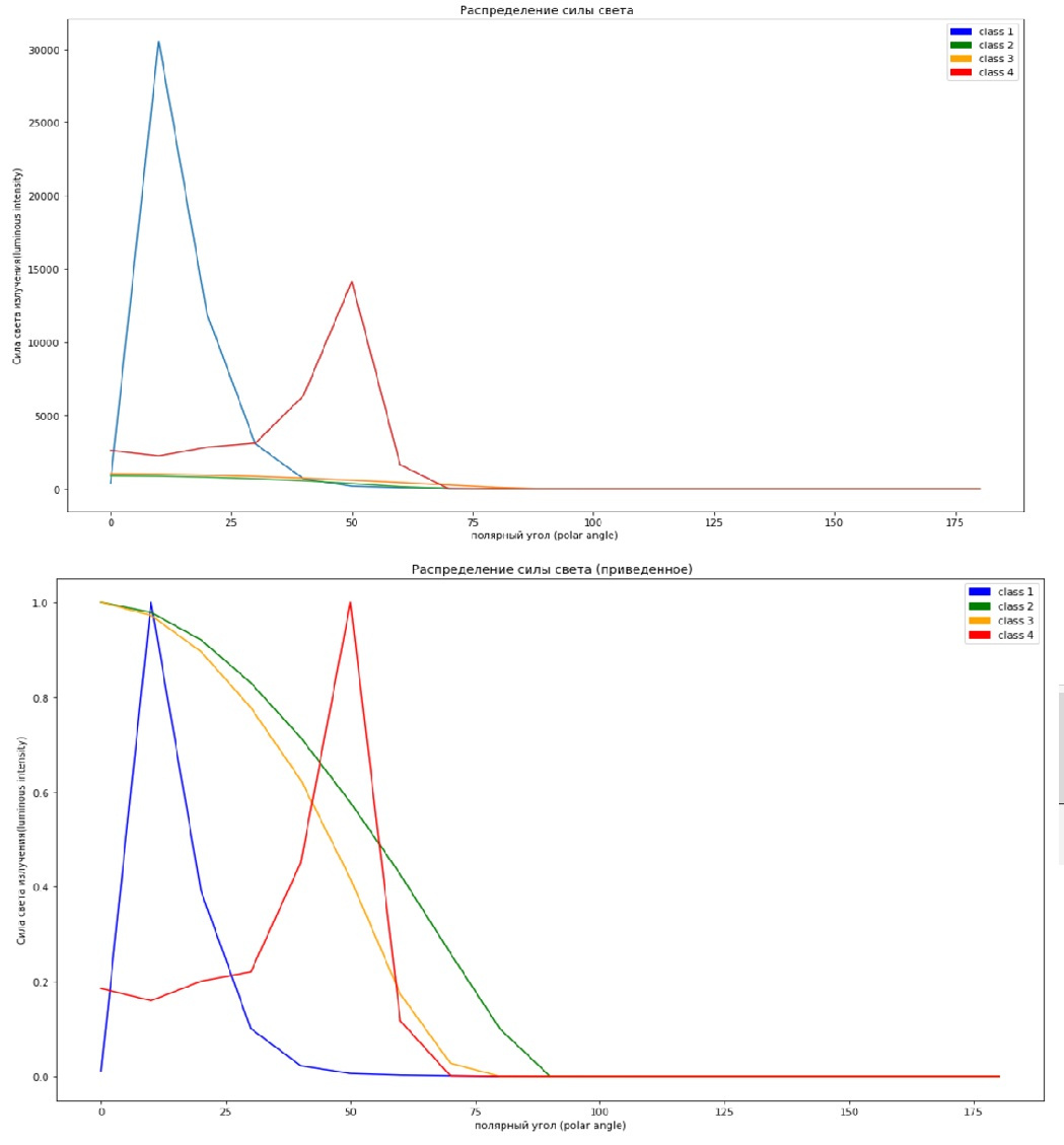 

The graphs show one sample from each class, and as we can see, it will be easier for us and the computer to understand something on the scaled graphics, because on the top some graphs simply merge with zero due to the difference in scale.



In order to finally make sure that we are right, let's try to reduce the dimension of the signs to two-dimensional, to display our data on two-dimensional graphs and see how much our data is separable (we will use t-SNE for this)

Left unscaled with scaling right

 #T-SNE colors = ["#190aff", "#0fff0f", "#ff641e" , "#ff3232"] tsne = TSNE(random_state=42) d_tsne = tsne.fit_transform(X_train) plt.figure(figsize=(10, 10)) plt.xlim(d_tsne[:, 0].min(), d_tsne[:, 0].max() + 10) plt.ylim(d_tsne[:, 1].min(), d_tsne[:, 1].max() + 10) for i in range(len(X_train)): #  ,       plt.text(d_tsne[i, 0], d_tsne[i, 1], str(y_train[i]), color = colors[y_train[i]-1], fontdict={'weight': 'bold', 'size': 10}) plt.xlabel("t-SNE feature 0") plt.ylabel("t-SNE feature 1") 

“Score” it in different cells (well, or make a subplot)

 #T-SNE for scaled data d_tsne = tsne.fit_transform(X_train_scl) plt.figure(figsize=(10, 10)) plt.xlim(d_tsne[:, 0].min(), d_tsne[:, 0].max() + 10) plt.ylim(d_tsne[:, 1].min(), d_tsne[:, 1].max() + 10) for i in range(len(X_train_scl)): #  ,       plt.text(d_tsne[i, 0], d_tsne[i, 1], str(y_train[i]), color = colors[y_train[i]-1], fontdict={'weight': 'bold', 'size': 10}) plt.xlabel("t-SNE feature 0") plt.ylabel("t-SNE feature 1") 

Subtract one, because I started counting tags not from scratch.







The figures show that on the scaled data, classes 1, 3, 4 are less well distinguished, and class 2 is spread between classes 1 and 3 (if you download and see KCC fixtures, you will understand that it should be so)

Episode VI: Return of the Jedi, or feel the power of models pre-written by someone for you!

Well, it's time to proceed to the direct classification.

First, let's teach SVC on our “truncated data”

 #predict part of full data (test labels the part of X_train) #not scaled svm = SVC(kernel= 'rbf', random_state=42 , gamma=2, C=1.1) svm.fit (X_train_part, y_train_part) pred=svm.predict(X_test_part) print("\n not scaled: \n results (pred, real): \n",list(zip(pred,y_test_part))) print('not scaled: accuracy = {}, f1-score= {}'.format( accuracy_score(y_test_part,pred), f1_score(y_test_part,pred, average='macro'))) #scaled svm = SVC(kernel= 'rbf', random_state=42 , gamma=2, C=1.1) svm.fit (X_train_part_scl, y_train_part) pred=svm.predict(X_test_part_scl) print("\n scaled: \n results (pred, real): \n",list(zip(pred,y_test_part))) print('scaled: accuracy = {}, f1-score= {}'.format( accuracy_score(y_test_part,pred), f1_score(y_test_part,pred, average='macro'))) 

We get the following conclusion



Not scaled

not scaled:

results (pred, real):

[(2, 3), (2, 3), (2, 2), (3, 3), (2, 1), (2, 3), (2, 3), (2, 2), (2, 1), (2, 2), (1, 1), (3, 3), (2, 2), (2, 1), (2, 4), (3, 3), (2, 2), (2, 4), (2, 1), (2, 2), (4, 4), (2, 2), (4, 4), (2, 4), (2, 3), (2, 1), (2, 1), (2, 1), (2, 2)]

not scaled: accuracy = 0.4827586206896552, f1-score= 0.46380859284085096



Scaled

scaled:

results (pred, real):

[(3, 3), (3, 3), (2, 2), (3, 3), (1, 1), (3, 3), (3, 3), (2, 2), (1, 1), (2, 2), (1, 1), (3, 3), (2, 2), (1, 1), (4, 4), (3, 3), (2, 2), (4, 4), (1, 1), (2, 2), (4, 4), (2, 2), (4, 4), (4, 4), (3, 3), (1, 1), (1, 1), (1, 1), (2, 2)]

scaled: accuracy = 1.0, f1-score= 1.0



As you can see, the difference is more than significant, if in the first case we managed to achieve

the results are only slightly better than the random prediction, then in the second case we received a 100% hit.



We will train our model on the complete data set and make sure that there will be a 100% result

 #final predict full data svm.fit (X_train_scl, y_train) pred=svm.predict(X_test_scl) print("\n results (pred, real): \n",list(zip(pred,y_test))) print('scaled: accuracy = {}, f1-score= {}'.format( accuracy_score(y_test,pred), f1_score(y_test,pred, average='macro'))) 

Let's look at the conclusion



results (pred, real):

[(1, 1), (1, 1), (1, 1), (1, 1), (1, 1), (1, 1), (1, 1), (1, 1), (1, 1), (1, 1), (1, 1), (1, 1), (1, 1), (2, 2), (2, 2), (2, 2), (2, 2), (2, 2), (2, 2), (2, 2), (2, 2), (2, 2), (2, 2), (2, 2), (2, 2), (2, 2), (3, 3), (3, 3), (3, 3), (3, 3), (3, 3), (3, 3), (3, 3), (3, 3), (3, 3), (3, 3), (3, 3), (3, 3), (3, 3), (4, 4), (4, 4), (4, 4), (4, 4), (4, 4), (4, 4), (4, 4), (4, 4), (4, 4)]

scaled: accuracy = 1.0, f1-score= 1.0



Perfect! It should be noted that, along with the accuracy metric, I decided to use the f1-score, which would have been useful to us if our classes had a significantly greater imbalance, but in our case there is almost no difference between the metrics (but we did see this clearly)



Well, the last thing we will check is the RandomForest classifier that is already familiar to us.

In books and other materials, I read that the scaling of features is not critical for RandomForest, let's see if this is so.

 rfc=RandomForestClassifier(random_state=42,n_jobs=-1, n_estimators=100) rfc=rfc.fit(X_train, y_train) rpred=rfc.predict(X_test) print("\n not scaled: \n results (pred, real): \n",list(zip(rpred,y_test))) print('not scaled: accuracy = {}, f1-score= {}'.format( accuracy_score(y_test,rpred), f1_score(y_test,rpred, average='macro'))) rfc=rfc.fit(X_train_scl, y_train) rpred=rfc.predict(X_test_scl) print("\n scaled: \n results (pred, real): \n",list(zip(rpred,y_test))) print('scaled: accuracy = {}, f1-score= {}'.format( accuracy_score(y_test,rpred), f1_score(y_test,rpred, average='macro'))) 

We get the following output:

not scaled:

results (pred, real):

[(1, 1), (1, 1), (2, 1), (1, 1), (1, 1), (2, 1), (1, 1), (1, 1), (1, 1), (1, 1), (1, 1), (1, 1), (1, 1), (2, 2), (2, 2), (2, 2), (1, 2), (2, 2), (2, 2), (2, 2), (2, 2), (3, 2), (2, 2), (3, 2), (2, 2), (4, 2), (3, 3), (3, 3), (3, 3), (3, 3), (3, 3), (3, 3), (3, 3), (3, 3), (3, 3), (3, 3), (4, 3), (3, 3), (3, 3), (4, 4), (4, 4), (4, 4), (4, 4), (4, 4), (4, 4), (4, 4), (4, 4), (4, 4)]

not scaled: accuracy = 0.8541666666666666, f1-score= 0.8547222222222222



scaled:

results (pred, real):

[(1, 1), (1, 1), (2, 1), (1, 1), (1, 1), (1, 1), (1, 1), (1, 1), (1, 1), (1, 1), (1, 1), (1, 1), (1, 1), (2, 2), (2, 2), (2, 2), (2, 2), (2, 2), (2, 2), (2, 2), (2, 2), (2, 2), (2, 2), (2, 2), (2, 2), (2, 2), (3, 3), (3, 3), (3, 3), (3, 3), (3, 3), (3, 3), (3, 3), (3, 3), (3, 3), (3, 3), (3, 3), (3, 3), (3, 3), (4, 4), (4, 4), (4, 4), (4, 4), (4, 4), (4, 4), (4, 4), (4, 4), (4, 4)]

scaled: accuracy = 0.9791666666666666, f1-score= 0.9807407407407408



So, we can make 2 conclusions:

1. Sometimes it is useful to scale the attributes even for decision trees.

2. SVC showed better accuracy.



It should be noted that this time I selected the parameters manually and if for scv I picked up the right option from the second attempt, I didn’t pick up Random from the 10th time, I spat and left it by default (except for the number of trees). Perhaps there are parameters that will bring the accuracy to 100%, try to pick up and be sure to tell in the comments.



Well, almost everything seems to be, but I think that Star Wars fans will not forgive me for not mentioning the seventh film of the saga, therefore ...

Episode VII: Awakening of power - instead of conclusion.

Machine learning turned out to be a damn fascinating thing, I still advise everyone to try to invent and solve a problem close to you.

Well, if something does not work right away, then do not hang your nose as in the picture below.







Yes Yes! So that you don’t think it is “hang your nose” and no other hidden thoughts;)



And may the force be with you!