ggplot2: how to easily combine multiple graphs in one, part 2
This article will show step by step how to combine several ggplot graphs in one or several illustrations using the helper functions available in the R ggpubr , cowplot and gridExtra packages . We also describe how to export the resulting graphs to a file.
We use the nested functions of
For example, the code below does the following:
')
The following combination of functions [from the cowplot package] can be used to place graphs at specific locations of a given size:
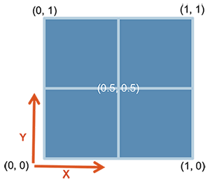
Note that by default, the coordinates vary from 0 to 1, and the point (0, 0) is in the lower left corner of the canvas (see illustration below).
Can work with label vectors with associated coordinates.
For example, you can combine several graphs of different sizes with a specific location:

The
For example, the code below does the following:
In
In the code below
You can also add annotation to the output of
To easily add annotations to the conclusions of
In the code above, we used
The grid package allows you to set a complex mutual arrangement of graphs using the
The steps can be described as:

To set a common legend for several ordered graphs, you can use the
In the next part:
Repositioning by row or column
Using the ggpubr package
We use the nested functions of
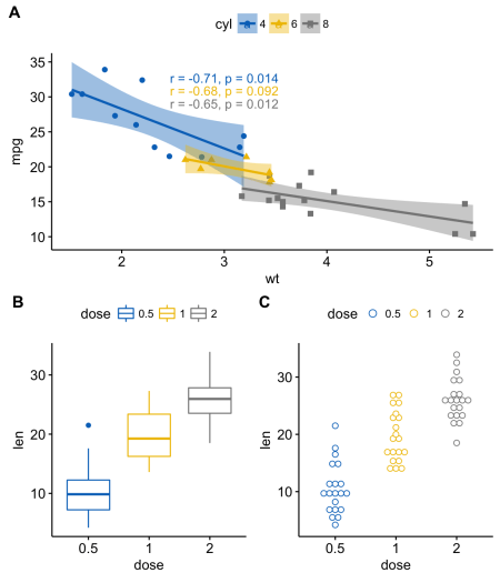
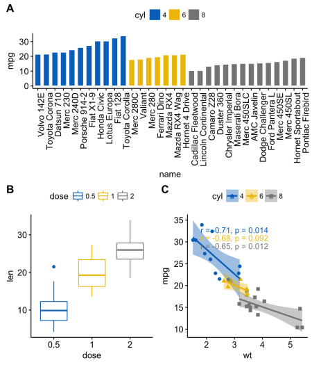
ggarrange() to change the location of the graphs in rows or columns.For example, the code below does the following:
- the scatter diagram (sp) will be in the first row and occupy two columns
- scatter diagram (bxp) and scatter diagram (dp) will occupy the second row and two different columns
ggarrange(sp, # ggarrange(bxp, dp, ncol = 2, labels = c("B", "C")), # nrow = 2, labels = "A" # ) ')
Use the cowplot package
The following combination of functions [from the cowplot package] can be used to place graphs at specific locations of a given size:
ggdraw() + draw_plot() + draw_plot_label() .ggdraw (). Initialize the blank canvas:
ggdraw() Note that by default, the coordinates vary from 0 to 1, and the point (0, 0) is in the lower left corner of the canvas (see illustration below).
draw_plot (). Has a schedule somewhere on the canvas:
draw_plot(plot, x = 0, y = 0, width = 1, height = 1) plot: plot to place (ggplot2 or gtable)x, y: x / y coordinates of the lower left corner of the graphwidth, height: the width and height of the graphic
draw_plot_label (). Adds a label in the upper right corner of the chart.
Can work with label vectors with associated coordinates.
draw_plot_label(label, x = 0, y = 1, size = 16, ...) label:labelvectorx, y: vector with x / y coordinates of each label, respectivelysize: label font size
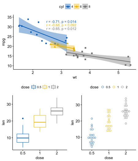
For example, you can combine several graphs of different sizes with a specific location:
library("cowplot") ggdraw() + draw_plot(bxp, x = 0, y = .5, width = .5, height = .5) + draw_plot(dp, x = .5, y = .5, width = .5, height = .5) + draw_plot(bp, x = 0, y = 0, width = 1, height = 0.5) + draw_plot_label(label = c("A", "B", "C"), size = 15, x = c(0, 0.5, 0), y = c(1, 1, 0.5)) Use the gridExtra package
The
arrangeGrop() function [in gridExtra ] helps to change the arrangement of graphs in rows or columns.For example, the code below does the following:
- the scatter diagram (sp) will be in the first row and occupy two columns
- scatter diagram (bxp) and scatter diagram (dp) will occupy the second row and two different columns
library("gridExtra") grid.arrange(sp, # arrangeGrob(bxp, dp, ncol = 2),# nrow = 2) # In
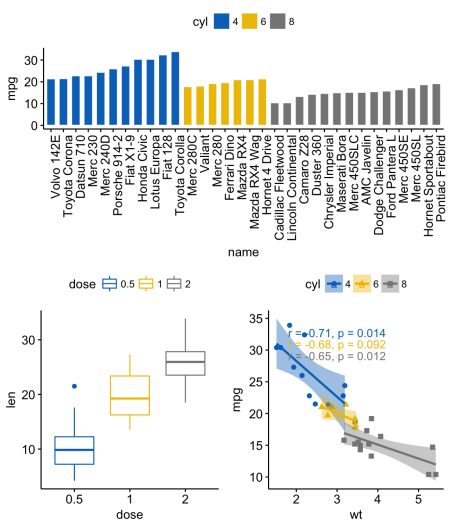
grid.arrange() you can also use the layout_matrix argument to create complex relative positioning of graphs.In the code below
layout_matrix is a 2x2 matrix (2 rows and 2 columns). The first line - all units, where the first chart occupies two columns; the second line contains graphs 2 and 3, each of which occupies its own column. grid.arrange(bp, # bxp, sp, # ncol = 2, nrow = 2, layout_matrix = rbind(c(1,1), c(2,3))) You can also add annotation to the output of
grid.arrange() using the auxiliary function draw_plot_label() [in cowplot ].To easily add annotations to the conclusions of
grid.arrange() or arrangeGrob() functions grid.arrange() arrangeGrob() type), you first need to convert them to ggplot type using the as_ggplot() function [in ggpubr ]. You can then use the draw_plot_label() function [in cowplot ]. library("gridExtra") library("cowplot") # arrangeGrob # gtable (gt) gt <- arrangeGrob(bp, # bxp, sp, # ncol = 2, nrow = 2, layout_matrix = rbind(c(1,1), c(2,3))) # p <- as_ggplot(gt) + # ggplot draw_plot_label(label = c("A", "B", "C"), size = 15, x = c(0, 0, 0.5), y = c(1, 0.5, 0.5)) # p In the code above, we used
arrangeGrob() instead of grid.arrange() . The main difference between these two functions is that grid.arrange() automatically displays ordered graphs. Since we wanted to add an annotation to the graphs before drawing them, it is preferable to use the arrangeGrob() function in this case.Use the grid package
The grid package allows you to set a complex mutual arrangement of graphs using the
grid.layout() function. It also provides the viewport() helper function for specifying a region, or scope. The print() function is used to place graphs in a given region.The steps can be described as:
- Create graphics: p1, p2, p3, ....
- Go to a new page using the
grid.newpage()function - Create location 2X2 - number of columns = 2; number of lines = 2
- Set scope: rectangular area on graphics device
- Print a graph in scope
library(grid) # grid.newpage() # : nrow = 3, ncol = 2 pushViewport(viewport(layout = grid.layout(nrow = 3, ncol = 2))) # define_region <- function(row, col){ viewport(layout.pos.row = row, layout.pos.col = col) } # print(sp, vp = define_region(row = 1, col = 1:2)) # print(bxp, vp = define_region(row = 2, col = 1)) print(dp, vp = define_region(row = 2, col = 2)) print(bp + rremove("x.text"), vp = define_region(row = 3, col = 1:2)) Using common legends for combined ggplot graphs
To set a common legend for several ordered graphs, you can use the
ggarrange() function [in ggpubr ] with these arguments:common.legend = TRUE: make a shared legendlegend: set the position of the legend. The allowed value is one of c (“top”, “bottom”, “left”, “right”)
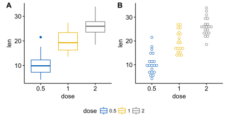
ggarrange(bxp, dp, labels = c("A", "B"), common.legend = TRUE, legend = "bottom") Scatter plot with unconditional density graphs
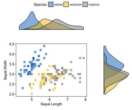
# , ("Species") sp <- ggscatter(iris, x = "Sepal.Length", y = "Sepal.Width", color = "Species", palette = "jco", size = 3, alpha = 0.6)+ border() # x ( ) y ( ) xplot <- ggdensity(iris, "Sepal.Length", fill = "Species", palette = "jco") yplot <- ggdensity(iris, "Sepal.Width", fill = "Species", palette = "jco")+ rotate() # yplot <- yplot + clean_theme() xplot <- xplot + clean_theme() # ggarrange(xplot, NULL, sp, yplot, ncol = 2, nrow = 2, align = "hv", widths = c(2, 1), heights = c(1, 2), common.legend = TRUE) In the next part:
- mix table, text and ggplot2 graphics
- add a graphic element to ggplot (table, scatterplot, background image)
- We have graphics on several pages.
- nested interposition
- export charts
Source: https://habr.com/ru/post/337598/
All Articles