We have already reviewed the PostgreSQL indexing mechanism , the access methods interface, and three methods: hash index , B-tree, and GiST . In this part, we will focus on the SP-GiST.

SP-GiST

First, a little about the title. The word "GiST" hints at a certain similarity with the method of the same name. The similarity is really there: both are generalized search trees, generalized search trees that provide a framework for building different access methods.



"SP" stands for space partitioning, a partition of space. The role of space is often exactly what we used to call space - for example, a two-dimensional plane. But, as we will see, any search space is meant , in fact, an arbitrary range of values.

')

SP-GiST is suitable for structures in which the space is recursively divided into disjoint regions. This class includes quadtree trees, k-dimensional trees (kD tree), prefix trees (trie).

Device

So, the idea of ​​the SP-GiST index method is to split a range of values ​​into non-overlapping subregions, each of which, in turn, can also be split. Such a partition generates unbalanced trees (as opposed to B-trees and regular GiST).



The non-intersection property simplifies decision making when inserting and searching. On the other hand, the resulting trees, as a rule, are weakly branchy. For example, a quad tree node usually has four child nodes (as opposed to B-trees, where they are measured in hundreds) and greater depth. Such trees are well suited for working in RAM, but the index is stored on disk, and therefore, to reduce the number of I / O operations, nodes have to be packed into pages — and this is not easy to do effectively. In addition, the search time for different values ​​in the index may differ due to the different depth of the branches.



Like GiST, this access method takes care of low-level tasks (simultaneous access and locking, logging, the search algorithm itself) and allows you to add support for new data types and partitioning algorithms, providing a special simplified interface for this.



The internal node of the SP-GiST tree stores references to child nodes; A label can be set for each link . In addition, the internal node can store a value called a prefix. In fact, this value does not have to be a prefix; it can be considered as an arbitrary predicate that runs for all child nodes.



SP-GiST leaf nodes contain the value of the indexed type and a link to the table row (TID). As the value, the indexed data itself can be used (search key), but not necessarily: the reduced value can also be stored.



In addition, leaf nodes can be listed. Thus, the internal node can refer not to a single value, but to the whole list.



Note that the prefixes, labels and values ​​in the leaf nodes can all be of completely different data types.



As in GiST, the main function to be defined for the search is the consistency function. This function is called for a tree node and returns a set of child nodes, the values ​​of which are “consistent” with the search predicate (as usual, of the form “ indexed-field operator expression ”). For a leaf node, the consistency function determines whether the indexed value in this node satisfies the search predicate.



The search begins at the root node. With the help of the consistency function, it becomes clear which subsidiaries it makes sense to enter; the algorithm is repeated for each of the found nodes. Search is made in depth.



At the physical level, index nodes are packed into pages so that they can be efficiently handled in terms of I / O operations. At the same time on the same page are either internal nodes, or leaf, but not both of them simultaneously.

Example: quad tree

A quadtree tree is used to index points on a plane. The idea is to recursively divide a region into four parts (quadrants) with respect to the central point. The depth of the branches of such a tree can vary and depends on the density of points in the corresponding quadrants.



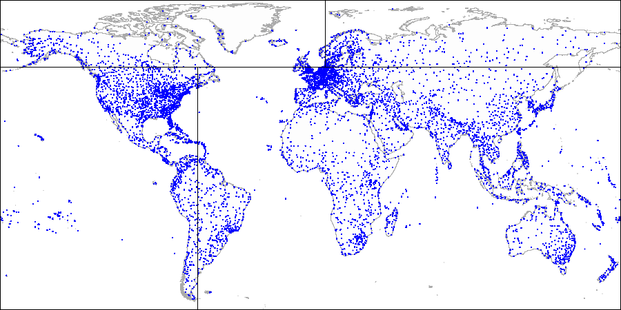
Here is how it looks in the pictures on the example of a demo database , supplemented by airports from the site openflights.org . By the way, we recently released a new version of the database, in which, among other things, we replaced longitude and latitude with a single field of type point.





First we divide the plane into four quadrants ...





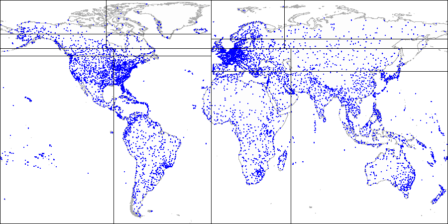
Then divide each of the quadrants ...





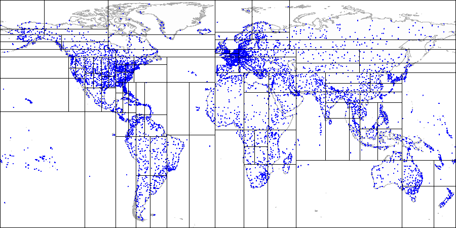
And so on, until we get the final split.



Let us now consider in more detail a simple example that we have already met in the part about GiST . Here’s what a plane partition might look like in this case:







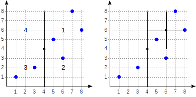
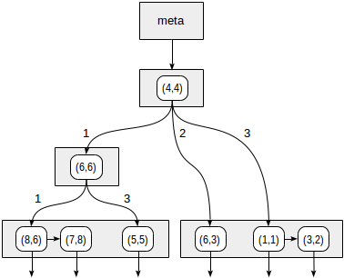
Quadrants are numbered as shown in the first figure; for definiteness, we will place the child nodes from left to right in exactly this sequence. A possible index structure in this case is shown in the figure below. Each internal node refers to a maximum of four child nodes. Each link can be labeled with a quadrant number, as shown. But there is no label implementation; it is more convenient to store a fixed array of four references, some of which may be empty.







The points lying on the borders belong to the quadrant with a smaller number.



postgres=# create table points(p point);

CREATE TABLE



postgres=# insert into points(p) values

(point '(1,1)'), (point '(3,2)'), (point '(6,3)'),

(point '(5,5)'), (point '(7,8)'), (point '(8,6)');

INSERT 0 6



postgres=# create index points_quad_idx on points using spgist(p);

CREATE INDEX



In this case, the default operator class is quad_point_ops, which includes the following operators:



postgres=# select amop.amopopr::regoperator, amop.amopstrategy

from pg_opclass opc, pg_opfamily opf, pg_am am, pg_amop amop

where opc.opcname = 'quad_point_ops'

and opf.oid = opc.opcfamily

and am.oid = opf.opfmethod

and amop.amopfamily = opc.opcfamily

and am.amname = 'spgist'

and amop.amoplefttype = opc.opcintype;

amopopr | amopstrategy

-----------------+--------------

<<(point,point) | 1

>>(point,point) | 5

~=(point,point) | 6

<^(point,point) | 10

>^(point,point) | 11

<@(point,box) | 8

(6 rows)



Consider, for example, how the query select * from points where p >^ point '(2,7)' will be executed (find all the points above the given one).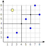







We start with the root node and choose which child nodes to descend using the consistency function. For the >^ operator >^ this function compares the point (2.7) with the central point of the node (4.4) and selects the quadrants at which the desired points may be located - in this case, the first and the fourth.



In the node corresponding to the first quadrant, we again determine the child nodes using the consistency function. The central point (6,6), and we again need to look through the first and fourth quadrants.







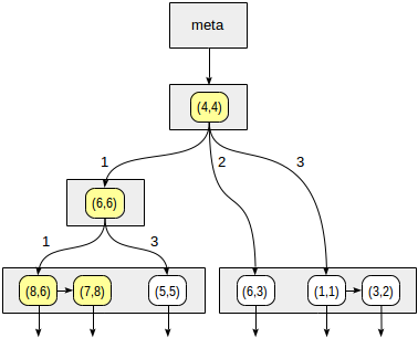
The first quadrant corresponds to the list of leaf nodes (8.6) and (7.8), of which only the point (7.8) fits the query condition. The reference to the fourth quadrant is empty.



At the internal node (4.4), the reference to the fourth quadrant is also empty, and the search is complete.



postgres=# set enable_seqscan = off;

SET

postgres=# explain (costs off) select * from points where p >^ point '(2,7)';

QUERY PLAN

------------------------------------------------

Index Only Scan using points_quad_idx on points

Index Cond: (p >^ '(2,7)'::point)

(2 rows)



Inside

The internal structure of the SP-GiST indexes can be studied using the gevel extension, which we have already talked about earlier. The bad news: due to an error, the extension does not work correctly on modern versions of PostgreSQL. Good news: we are planning to transfer the gevel functionality to pageinspect ( discussion ). And the error is already fixed there.



For example, take the extended demo database, which was used to draw pictures with a map of the world.



demo=# create index airports_coordinates_quad_idx on airports_ml using spgist(coordinates);

CREATE INDEX



About the index, you can, firstly, find out some statistical information:



demo=# select * from spgist_stats('airports_coordinates_quad_idx');

spgist_stats

----------------------------------

totalPages: 33 +

deletedPages: 0 +

innerPages: 3 +

leafPages: 30 +

emptyPages: 2 +

usedSpace: 201.53 kbytes+

usedInnerSpace: 2.17 kbytes +

usedLeafSpace: 199.36 kbytes+

freeSpace: 61.44 kbytes +

fillRatio: 76.64% +

leafTuples: 5993 +

innerTuples: 37 +

innerAllTheSame: 0 +

leafPlaceholders: 725 +

innerPlaceholders: 0 +

leafRedirects: 0 +

innerRedirects: 0

(1 row)



And second, output the index tree itself:



demo=# select tid, n, level, tid_ptr, prefix, leaf_value

from spgist_print('airports_coordinates_quad_idx') as t(

tid tid,

allthesame bool,

n int,

level int,

tid_ptr tid,

prefix point, --

node_label int, -- ( )

leaf_value point --

)

order by tid, n;

tid | n | level | tid_ptr | prefix | leaf_value

---------+---+-------+---------+------------------+------------------

(1,1) | 0 | 1 | (5,3) | (-10.220,53.588) |

(1,1) | 1 | 1 | (5,2) | (-10.220,53.588) |

(1,1) | 2 | 1 | (5,1) | (-10.220,53.588) |

(1,1) | 3 | 1 | (5,14) | (-10.220,53.588) |

(3,68) | | 3 | | | (86.107,55.270)

(3,70) | | 3 | | | (129.771,62.093)

(3,85) | | 4 | | | (57.684,-20.430)

(3,122) | | 4 | | | (107.438,51.808)

(3,154) | | 3 | | | (-51.678,64.191)

(5,1) | 0 | 2 | (24,27) | (-88.680,48.638) |

(5,1) | 1 | 2 | (5,7) | (-88.680,48.638) |

...



But keep in mind. that the spgist_print function does not display all leaf values, but only the first one from the list, and therefore shows the structure of the index, and not its full content.

Example: k-dimensional trees

For the same points on the plane, we can offer another way of splitting the space.



Let's draw a horizontal line through the first point to be indexed . It breaks the plane into two parts: upper and lower. The second index point falls into one of these parts. Through it we draw a vertical line that breaks this part into two: right and left. Through the next point we again draw a horizontal line, through the next - a vertical line and so on.



All internal nodes of a tree constructed in this way will have only two child nodes. Each of the two links can lead either to the next internal node in the hierarchy, or to the list of leaf nodes.



The method is easily generalized to k-dimensional spaces, therefore trees in the literature are called k-dimensional (kD tree).



For example airports:





First we divide the plane into top and bottom ...





Then each part to the left and right ...





And so on, until we get the final split.



To use such a partition, you must explicitly specify the kd_point_ops operator class when creating an index:



postgres=# create index points_kd_idx on points using spgist(p kd_point_ops );

CREATE INDEX





This class includes exactly the same operators as the “default” quad_point_ops.

Inside

When viewing the tree structure, one should take into account that the prefix in this case is not a point, but only one coordinate:



demo=# select tid, n, level, tid_ptr, prefix, leaf_value

from spgist_print('airports_coordinates_kd_idx') as t(

tid tid,

allthesame bool,

n int,

level int,

tid_ptr tid,

prefix float, --

node_label int, -- ( )

leaf_value point --

)

order by tid, n;

tid | n | level | tid_ptr | prefix | leaf_value

---------+---+-------+---------+------------+------------------

(1,1) | 0 | 1 | (5,1) | 53.740 |

(1,1) | 1 | 1 | (5,4) | 53.740 |

(3,113) | | 6 | | | (-7.277,62.064)

(3,114) | | 6 | | | (-85.033,73.006)

(5,1) | 0 | 2 | (5,12) | -65.449 |

(5,1) | 1 | 2 | (5,2) | -65.449 |

(5,2) | 0 | 3 | (5,6) | 35.624 |

(5,2) | 1 | 3 | (5,3) | 35.624 |

...



Example: prefix tree

With SP-GiST, you can implement a prefix tree (radix tree) for strings. The idea of ​​a prefix tree is that the row being indexed is not stored entirely in the leaf node, but is obtained by concatenating the values ​​stored in the nodes up from the given to the root.



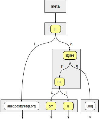
Suppose you need to index the addresses of sites: “postgrespro.ru”, “postgrespro.com”, “postgresql.org” and “planet.postgresql.org”.



postgres=# create table sites(url text);

CREATE TABLE



postgres=# insert into sites values ('postgrespro.ru'),('postgrespro.com'),('postgresql.org'),('planet.postgresql.org');

INSERT 0 4



postgres=# create index on sites using spgist(url);

CREATE INDEX



The tree will look like this:







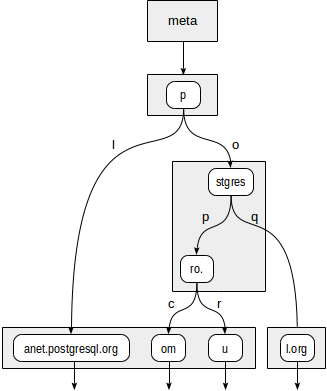
In the internal nodes of the tree are stored prefixes that are common to all child nodes. For example, in the daughters of the “stgres” node, the values ​​begin with “p” + “o” + “stgres”.



Each pointer to a child node, unlike the quad tree, is additionally marked with one character (in fact, two bytes, but this is not so important).



The text_ops operator class supports b-tree operators: “equal”, “more”, “less”:



postgres=# select amop.amopopr::regoperator, amop.amopstrategy

from pg_opclass opc, pg_opfamily opf, pg_am am, pg_amop amop

where opc.opcname = 'text_ops'

and opf.oid = opc.opcfamily

and am.oid = opf.opfmethod

and amop.amopfamily = opc.opcfamily

and am.amname = 'spgist'

and amop.amoplefttype = opc.opcintype;

amopopr | amopstrategy

-----------------+--------------

~<~(text,text) | 1

~<=~(text,text) | 2

=(text,text) | 3

~>=~(text,text) | 4

~>~(text,text) | 5

<(text,text) | 11

<=(text,text) | 12

>=(text,text) | 14

>(text,text) | 15

(9 rows)



Operators with tildes differ in that they work not with characters, but with bytes.



In some cases, the representation in the form of a prefix tree may turn out to be much more compact than the B-tree due to the fact that the values ​​are not stored as a whole, but are reconstructed as necessary when moving along the tree.



Consider the query: select * from sites where url like 'postgresp%ru' . It can be performed using an index:



postgres=# explain (costs off) select * from sites where url like 'postgresp%ru';

QUERY PLAN

------------------------------------------------------------------------------

Index Only Scan using sites_url_idx on sites

Index Cond: ((url ~>=~ 'postgresp'::text) AND (url ~<~ 'postgresq'::text))

Filter: (url ~~ 'postgresp%ru'::text)

(3 rows)



In fact, the index contains values ​​greater than or equal to “postgresp” and at the same time smaller “postgresq” (Index Cond), and then the appropriate values ​​are selected from the result (Filter).



First, the consistency function must decide which children of the root “p” need to descend. There are two options: "p" + "l" (does not fit, even without looking further) and "p" + "o" + "stgres" (suitable).



The “stgres” node again requires a call to the consistency function to check for “postgres” + “p” + “ro.” (Suitable) and “postgres” + “q” (not suitable).



For the “ro.” Node and all its child leaf nodes of the consistency function, the answer is “suitable”, so the index method returns two values: “postgrespro.com” and “postgrespro.ru”. From them - already at the stage of filtration - one suitable value will be chosen.

Inside

When viewing the tree structure, you need to consider the data types:



postgres=# select * from spgist_print('sites_url_idx') as t(

tid tid,

allthesame bool,

n int,

level int,

tid_ptr tid,

prefix text, --

node_label smallint, --

leaf_value text --

)

order by tid, n;



Properties

Let's take a look at the properties of the spgist access method (requests were given earlier ):



amname | name | pg_indexam_has_property

--------+---------------+-------------------------

spgist | can_order | f

spgist | can_unique | f

spgist | can_multi_col | f

spgist | can_exclude | t





SP-GiST indices cannot be used to sort and maintain uniqueness. In addition, such indexes cannot be built on several columns (unlike GiST). Use to support exception restrictions is allowed.



Index properties:



name | pg_index_has_property

---------------+-----------------------

clusterable | f

index_scan | t

bitmap_scan | t

backward_scan | f



Here, the difference from GiST is the lack of clustering.



And finally, the properties of the column level:



name | pg_index_column_has_property

--------------------+------------------------------

asc | f

desc | f

nulls_first | f

nulls_last | f

orderable | f

distance_orderable | f

returnable | t

search_array | f

search_nulls | t



There is no support for sorting, which is understandable. Distance operators for finding nearest neighbors in SP-GiST are not yet available; most likely such support will appear in the future.



SP-GiST can be used exclusively for index scanning, at least for the operator classes considered. As we have seen, in some cases, indexed values ​​are directly stored in leaf nodes, and in some cases they are restored in parts as they descend through a tree.

Undefined values

So far, we have not said anything about uncertain values ​​in order not to complicate the picture. As can be seen from the properties of the index, NULL is supported. And really:



postgres=# explain (costs off)

select * from sites where url is null;

QUERY PLAN

----------------------------------------------

Index Only Scan using sites_url_idx on sites

Index Cond: (url IS NULL)

(2 rows)



However, the indefinite value for SP-GiST is something alien. All operators in the spgist class of operators must be strict: for undefined parameters, they must return an undefined result. This is provided by the method itself; undefined values ​​are simply not passed to operators.



But, in order for the access method to be used exclusively for index scanning, the undefined values ​​must still be stored in the index. They are stored, but in a separate tree with its own root.

Other data types

In addition to points and prefix trees for strings, other methods based on SP-GiST are implemented in PostgreSQL:

• A quad tree for rectangles provides a class of box_ops operators.
  
  Each rectangle is represented by a point in four-dimensional space, so the number of quadrants is 16. Such an index can win GiST in performance, when there are many intersections among rectangles: in GiST it is impossible to draw boundaries so as to separate intersecting objects from each other, but with points albeit four-dimensional) there are no such problems.
  
  
• The quad tree for ranges provides the range_ops operator class.
  
  The interval is represented by a two-dimensional point: the lower bound becomes the abscissa, and the upper bound - the ordinate.
  
  

Continued .