Using Python to process real-time information from sensors that work with Arduino
Formulation of the problem
Digital and analog sensors connected to the Arduino, generate large amounts of information that requires processing in real time [1].
Currently, data from Arduino is printed from the command line or displayed in a graphical user interface with delay. Therefore, real-time data is not stored, which makes it impossible to analyze them further.
This publication is devoted to a software solution to the problem of storing information from sensors working with Arduino and its graphical representation in real time. The examples are used by well-known sensors, such as a potentiometer and a PIR motion sensor.
')
Using CSV files to store data received from sensors working with Arduino
- You can use a simple listing to write data to a CSV file:
import csv data = [[1, 2, 3], ['a', 'b', 'c'], ['Python', 'Arduino', 'Programming']] with open('example.csv', 'w') as f: w = csv.writer (f) for row in data: w.writerow(row) - You can use the following listing to read data from a CSV file:
import csv with open('example.csv', 'r') as file: r = csv.reader(file) for row in r: print(row)
Consider saving the Arduino data on the example of two sensors - a potentiometer with an analog output signal and movement (PIR) with a digital output signal.
The potentiometer is connected to analog output 0, and the PIR motion sensor to digital output 11, as shown in the following diagram:
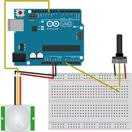
For this scheme to work, you need to load the pyFirmata module and the StandardFirmata sketch into the Arduino board in Python.
In any Python file, place the following code that starts and stops writing data from both sensors to the SensorDataStore.csv file:
Listing No. 1
#!/usr/bin/python import csv import pyfirmata from time import sleep port = 'COM3' board = pyfirmata.Arduino(port) it = pyfirmata.util.Iterator(board) it.start() pirPin = board.get_pin('d:11:i') a0 = board.get_pin('a:0:i') print(pirPin) with open('SensorDataStore.csv', 'w+') as f: w = csv.writer(f) w.writerow(["Number", "Potentiometer", "Motion sensor"]) i = 0 pirData = pirPin.read() m=25 n=1 while i < m: sleep(1) if pirData is not None: i += 1 potData = a0.read() pirData = pirPin.read() row = [i, potData, pirData] print(row) w.writerow(row) print ("Done. CSV file is ready!") board.exit() As a result of Listing No. 1, we get the data record in the 'SensorDataStore.csv' file:

Consider the code associated with the storage of sensor data. The first line of the entry in the CSV file is a header line that explains the contents of the columns: w.writerow (["Number", "Potentiometer", "Motion sensor"]) .
When the data change dynamics appears, which for the given scheme can be artificially created by turning the potentiometer knob or moving the hand near the motion sensor, the number of records in the data file becomes critical. To restore the waveform, the frequency of writing data to a file must be twice as large as the frequency of the signal change. The step n can be used to adjust the recording frequency, and the number of cycles to adjust the measurement time is m. However, the limitations on n below impose the speed of the sensors themselves. This function in the program above is performed by the following code fragment:
m=25 n=1 while i < m: sleep(n) if pirData is not None: i += 1 row = [i, potData, pirData] w.writerow (row) The given programs may be modified in accordance with the design requirements as follows:
- You can change the Arduino pin numbers and the number of pins to be used. This can be done by adding additional values for new sensors to the Python code and the StandardFirmata standard Arduino sketch.
- CSV file: the file name and location can be changed from SensorDataStore.csv to one that relates to your application.
- The frequency of m records in the SensorDataStore.csv file can be changed by changing the step, and the duration of the record by changing the number of cycles at a constant step.
Graphical analysis of data from a CSV file
Using the SensorDataStore.csv file, we will create a program for teaching data arrays from a potentiometer and a motion sensor and plotting data from these arrays:
Listing 2
import sys, csv import csv from matplotlib import pyplot i = [] mValues = [] pValues = [] with open('SensorDataStore.csv', 'r') as f: reader = csv.reader(f) header = next(reader, None) for row in reader: i.append(int(row[0])) pValues.append(float(row[1])) if row[2] == 'True': mValues.append(1) else: mValues.append(0) pyplot.subplot(2, 1, 1) pyplot.plot(i, pValues, '-') pyplot.title('Line plot - ' + header[1]) pyplot.xlim([1, 25]) pyplot.xlabel('X Axis') pyplot.ylabel('Y Axis') pyplot.subplot(2, 1, 2) pyplot.bar(i, mValues) pyplot.title('Bar chart - ' + header[2]) pyplot.xlim([1, 25]) pyplot.xlabel('X Axis') pyplot.ylabel('Y Axis') pyplot.tight_layout() pyplot.show() As a result of Listing 2, we will get two graphs on one form for displaying in real time the output data of a potentiometer and a motion sensor.
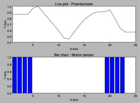
In this program, we created two sensor value arrays - pValues and mValues - by reading the SensorDataStore.csv file in rows. Here, pValues and mValues represent sensor data for the potentiometer and the motion sensor, respectively. Using the matplotlib methods , we construct two graphs on one form.
The generated code after each cycle of forming data arrays pValues and mValues received from the Arduino sensors updates the interface, which allows to conclude that the data was received in real time.
However, the method of storing and visualizing data has the following features: the entire data set is first written to the SensorDataStore.csv file (Listing 1), and then read from this file (Listing 2). Charts should be redrawn every time new values from Arduino arrive. Therefore, it is necessary to develop a program in which the planning and updating of graphs occurs in real time, and the entire set of sensor values is not built, as in listings No. 1.2. [2].
We write a program for a potentiometer creating the dynamics of the output signal by changing its active resistance to direct current.
Listing 3
import sys, csv from matplotlib import pyplot import pyfirmata from time import sleep import numpy as np # Associate port and board with pyFirmata port = '/dev/cu.usbmodemfa1321' board = pyfirmata.Arduino(port) # Using iterator thread to avoid buffer overflow it = pyfirmata.util.Iterator(board) it.start() # Assign a role and variable to analog pin 0 a0 = board.get_pin(''a:0:i'') # Initialize interactive mode pyplot.ion() pData = [0] * 25 fig = pyplot.figure() pyplot.title(''Real-time Potentiometer reading'') ax1 = pyplot.axes() l1, = pyplot.plot(pData) pyplot.ylim([0,1]) # real-time plotting loop while True: try: sleep(1) pData.append(float(a0.read())) pyplot.ylim([0, 1]) del pData[0] l1.set_xdata([i for i in xrange(25)]) l1.set_ydata(pData) # update the data pyplot.draw() # update the plot except KeyboardInterrupt: board.exit() break As a result of Listing 3, we will get a schedule.

Real-time planning in this exercise is achieved using a combination of the functions pyplot ion (), draw (), set_xdata () and set_data () . The ion () method initializes the pyplot interactive mode. The interactive mode helps to dynamically change the x and y values of the graphs in the pyplot.ion () picture.
When the interactive mode is set to True , a graph will appear only when the draw () method is called. We initialize the Arduino board using the pyFirmata module and input pins for obtaining sensor values.
As you can see in the next line of code, after setting up the Arduino board and the pyplot interactive mode, we initialized the graph with a set of empty data, in our case 0: pData = [0] * 25 .
This array for y values, pData , is then used to add values from the sensor in a while loop . The while loop continues to add new values to this data array and redraws the graph with these updated arrays for x and y values.
In Listing 3, we add new sensor values at the end of the array, while at the same time removing the first element of the array to limit the size of the array:
pData.append(float(a0.read())) del pData[0] The set_xdata () and set_ydata () methods are used to update the x and y axis data from these arrays. These updated values are plotted using the draw () method at each iteration of the while loop :
l1.set_xdata([i for i in xrange(25)]) l1.set_ydata(pData) # update the data pyplot.draw() # update the plot You will also notice that we use the xrange () function to generate a range of values according to the length provided, which is 25 in our case. The code fragment [i for i in xrange (25)] will generate a list of 25 integers, which begin gradually from 0 and end in 24.
Integration of graphs in the Tkinter window
Thanks to the powerful features of Python integration, it is very convenient to link the graphics created by the matplotlib library to the Tkinter GUI. We write a program for the connection between Tkinter and matplotlib .
Listing 4
import sys from matplotlib import pyplot import pyfirmata from time import sleep import Tkinter def onStartButtonPress(): while True: if flag.get(): sleep(1) pData.append(float(a0.read())) pyplot.ylim([0, 1]) del pData[0] l1.set_xdata([i for i in xrange(25)]) l1.set_ydata(pData) # update the data pyplot.draw() # update the plot top.update() else: flag.set(True) break def onPauseButtonPress(): flag.set(False) def onExitButtonPress(): print "Exiting...." onPauseButtonPress() board.exit() pyplot.close(fig) top.quit() top.destroy() print "Done." sys.exit() # Associate port and board with pyFirmata port = 'COM4' board = pyfirmata.Arduino(port) # Using iterator thread to avoid buffer overflow it = pyfirmata.util.Iterator(board) it.start() # Assign a role and variable to analog pin 0 a0 = board.get_pin('a:0:i') # Tkinter canvas top = Tkinter.Tk() top.title("Tkinter + matplotlib") # Create flag to work with indefinite while loop flag = Tkinter.BooleanVar(top) flag.set(True) pyplot.ion() pData = [0.0] * 25 fig = pyplot.figure() pyplot.title('Potentiometer') ax1 = pyplot.axes() l1, = pyplot.plot(pData) pyplot.ylim([0, 1]) # Create Start button and associate with onStartButtonPress method startButton = Tkinter.Button(top, text="Start", command=onStartButtonPress) startButton.grid(column=1, row=2) # Create Stop button and associate with onStopButtonPress method pauseButton = Tkinter.Button(top, text="Pause", command=onPauseButtonPress) pauseButton.grid(column=2, row=2) # Create Exit button and destroy the window exitButton = Tkinter.Button(top, text="Exit", command=onExitButtonPress) exitButton.grid(column=3, row=2) top.mainloop() As a result of listing No. 4, we get the Tkinter built into the window. the chart with button interface elements is startButton, pauseButton and exitButton.
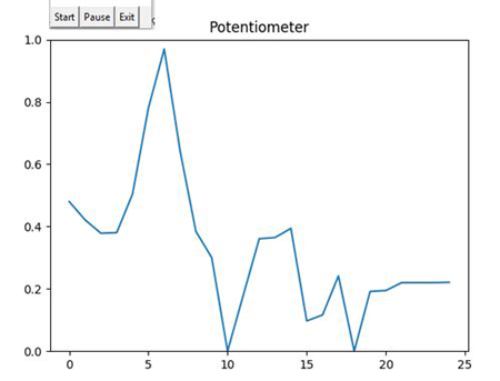
The “Start” and “Exit” buttons provide control points for matplotlib operations, such as updating the schedule and closing the schedule using the corresponding onStartButtonPress () and onExitButtonPress () functions. The onStartButtonPress () function also consists of the interaction point between the matplotlib and pyFirmata libraries . As you can see from the following code snippet, we will begin to update the graph using the draw () method and the Tkinter window using the update () method for each observation with analog output a0 , which is obtained using the read () method.
The onExitButtonPress () function implements the exit function, as described in the name itself. It closes the pyplot shape and the Tkinter window before disconnecting the Arduino board from the serial port.
After making the appropriate changes to the Arduino port parameter, start listing No. 4. You should see a window on the screen similar to the one shown in the previous screenshot. With this code, you can now manage real-time graphs using the “Start” and “Pause” buttons. Press the “Start” button and start rotating the potentiometer knob. When you press the “Pause” button, you may notice that the program has stopped building new values. When you press the Pause button, even rotating the knob will not lead to any changes in the graph.
As soon as you press the “Start” button again, you will see again that the schedule is updated in real time, discarding the values generated during the pause. Click the "Exit" button to safely close the program.
In preparing the materials of this publication participated Misov O. P.
findings
This publication presents two basic Python programming paradigms: creating, reading and writing files using Python, and storing data in these files and building sensor values and updating real-time graphs. We also learned how to store and display Arduino sensor data in real time. In addition to helping you with Arduino projects, these methods can also be used in everyday Python projects.
Links
Source: https://habr.com/ru/post/337494/
All Articles