How we taught the Yandex.Taxi application to predict a destination
Imagine: you open the app to once again order a taxi to the place you often visit, and, of course, in 2017 you expect that all you need to do is to say “Call”, and the taxi will immediately leave you. And where you wanted to go, in how many minutes and on which machine - all this application will learn thanks to the history of orders and machine learning. In general, everything is like in jokes about the perfect interface with a single button “do well”, better than which only the screen with the words “everything is already well”. It sounds great, but how to bring this reality closer?

The other day we released a new application Yandex. Taxi for iOS. In the updated interface, one of the accents is made on the choice of the end point of the route (“point B”). But the new version is not just a new UI. By the launch of the update, we significantly reworked the destination forecasting technology, replacing the old heuristics with a classifier trained on historical data.
')
As you understand, the buttons “do well” in machine learning are not there either, so a seemingly simple task turned into a rather exciting case, as a result of which, we hope, we managed to make life a little easier for users. Now we continue to closely monitor the work of the new algorithm and will continue to change it so that the quality of the forecast is more stable. At full capacity, we will launch in the next few weeks, but under the cut are already ready to talk about what is happening inside.
When choosing a destination, in the “where” field we have the opportunity to offer the user literally 2-3 options on the main screen and several more - if he goes to the point B selection menu:

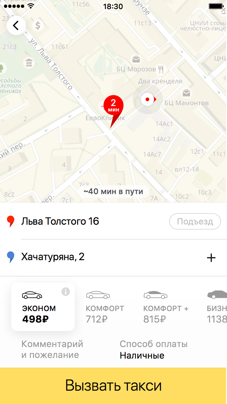

If our prediction is correct, the user does not need to type in the address, and in general there is reason to rejoice that the application is able to remember at least a little its preferences. It was for these prompts that a model was developed which, based on the user's travel history, tries to predict exactly where he is most likely to go now.
Before building a model based on machine learning, the following strategy was implemented: all points from the history are taken, “identical” points (with the same address or close) merge, different points are given different points for different locations (if the user went to this point, he went from this point, went to this point in some time window, and so on). Then the locations with the highest points are selected and recommended to the user. As I have already said, historically this strategy worked well, but the prediction accuracy could be improved. And most importantly - we knew how.
Our task was to use the re-ranking of the most probable “points B” on top of the “old” strategy using machine learning. The general approach is this: first, we award points, as before, then we take the top n for these points (where n is obviously more than what we need to recommend), and then re-rank it and the user will only show the three most likely points B. Exact number The candidates in the list are, of course, determined in the course of optimization so that both the quality of candidates and the quality of re-ranking are as high as possible. In our case, the optimal number of candidates turned out to be 20.
First, the quality must be divided into two parts: the quality of candidates and the quality of ranking. The quality of candidates is how well selected candidates are, in principle, correctly rearranged. And the quality of ranking is how well we predict the destination point, provided that it is among the candidates.
Let's start with the first metric, that is, the quality of candidates. It is worth noting that only about 72 percent of orders selected point B (or very close to it geographically) was present earlier in history. This means that the maximum quality of candidates is limited to this number, since we cannot yet recommend points to which a person has never traveled. We selected heuristics with assignment of points so that when selecting the top 20 candidates for these points the correct answer was contained in 71% of cases. With a maximum of 72%, this is a very good result. We were completely satisfied with this quality of candidates, so we didn’t touch this part of the model, although, in principle, we could. For example, instead of heuristics, it was possible to train a separate model. But since the heuristics-based search engine has already been technically implemented, we were able to save on development only by selecting the necessary coefficients.
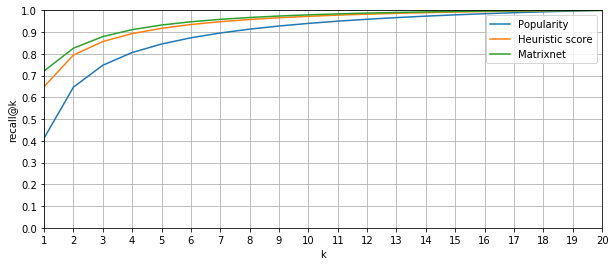
Let's go back to the quality of re-ranking. Since we can show one, two, or a maximum of three points on the main screen of the trip order, we are interested in the proportion of cases when the correct answer was in the top-1, top-2 and top-3 ranking lists, respectively. In machine learning, the share of correct answers in the top k of the ranking list (of all correct answers) is called recall @ k. In our case, we are interested in recall @ 1, recall @ 2 and recall @ 3. In this case, the “correct answer” in our problem is only one (up to closely spaced points), which means that this metric will just show the proportion of cases when the real “point B” falls in the top 1, top 2 and top 3 of our algorithm .
As a basic ranking algorithm, we took the sort by the number of points and obtained the following results (in percent): recall @ 1 = 63.7; Recalling @ 2 = 78.5 and recall @ 3 = 84.6. Note that the percentages here are a fraction of those cases where the correct answer in the candidates was generally present . At some point a logical question arose: perhaps simple sorting by popularity already gives good quality, and all the ideas of sorting by points and using machine learning are superfluous? But no, such an algorithm showed the worst quality: recall @ 1 = 41.2; recall @ 2 = 64.6; recall @ 3 = 74.7.
Remember the original results and proceed to discuss the machine learning model.
To begin, we describe the mechanism for finding candidates. As we have already said, on the basis of statistics on user’s trips to different places, points are awarded. A point earns points if trips are made to or from it; and significantly more points get those points to which the user traveled from the place where he is now, and even more points if this happened around the same time. Further, the logic is clear.
We now turn to the model for re-ranking. Since we want to maximize recall @ k, in the first approximation we want to predict the likelihood of the user going to a certain place and rank the places by probability. “As a first approximation,” because these arguments are true only with a very accurate estimate of probabilities, and when errors appear in them, recall @ k can be better optimized by another solution. A simple analogy: in machine learning, if we know for sure all probability distributions, the best classifier is Bayesian , but since in practice distributions are reconstructed from data approximately, often other classifiers work better.
The classification task was posed as follows: the objects were couples (history of the user's previous trips; candidate for recommendations), where positive examples (class 1) were couples in which the user did go to this point B, negative examples (class 0) were pairs in which the user eventually went to another place.
Thus, if you were a hardened formalist, the model did not estimate the likelihood that a person would go to a specific point, but the shifted probability that a given “story-candidate” pair is relevant. However, sorting by this value is as meaningful as sorting by the probability of a trip to a point. It can be shown that with an excess of data, these will be equivalent sorts.
We trained the classifier to minimize log loss, and as a model, we used the Matrixnet actively used in Yandex (gradient boosting over decision trees). And if everything is clear with MatrixNet, then why was log loss optimized?
Well, first, the optimization of this metric leads to the correct estimates of probability. The reason why this happens is rooted in mathematical statistics, in the maximum likelihood method . Let the probability of a single class at the i-th object be pi and the true class is yi . Then, if we consider the outcomes independent, the likelihood of the sample (roughly speaking, the probability of obtaining exactly the outcome that was obtained) is equal to the following product:
Secondly, we, of course, trust the theory, but just in case, we tried to optimize various loss functions, and the log loss showed the largest recall @ k, so everything eventually came together.
We talked about the method, the function of the error, too, one important detail remained: the signs by which we trained our classifier. We used more than a hundred different signs to describe each “history candidate” pair. Here are some examples:

And finally, about the results: after re-ranking using the model we built, we obtained the following data (again, in percent): recall @ 1 = 72.1 (+8.4); recall @ 2 = 82.6 (+4.1); recall @ 3 = 88 (+3,4). Not bad at all, but improvements are possible in the future due to the inclusion of additional information in the signs.
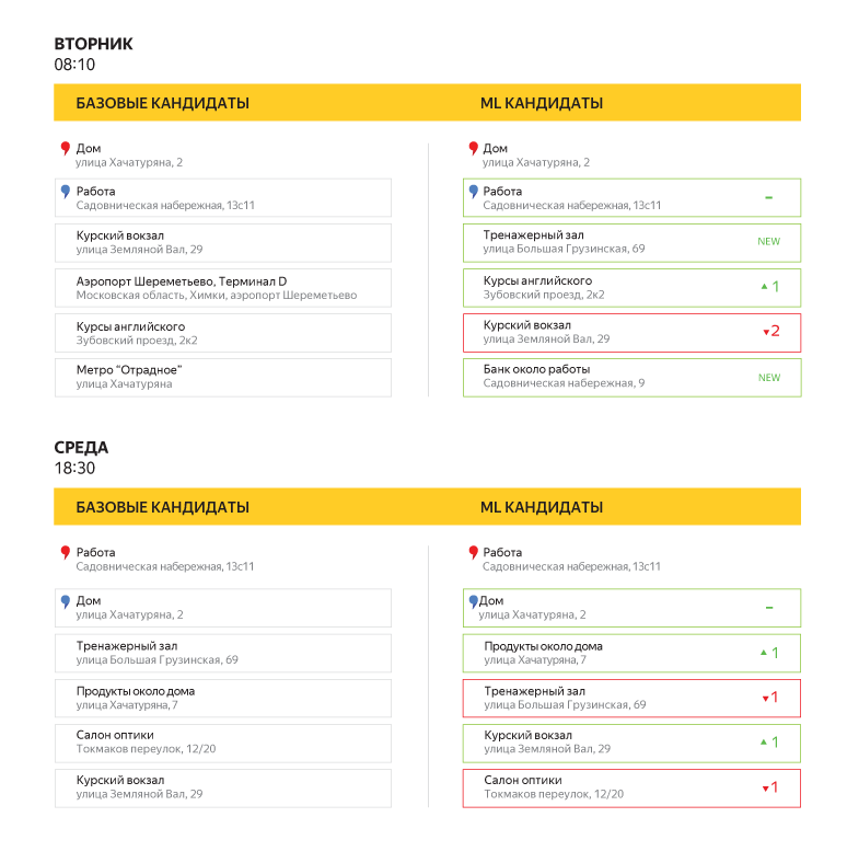
You can look at an example of how the new prediction algorithm will look to the user:
Of course, there are many experiments to improve the model. There will be the addition of new data to build recommendations, including the interests of the user, as well as the alleged “home” and “work” from Yandex Crypt and related features, and an experiment comparing the various classification methods in this task. For example, Yandex already has not only used exclusively within the MatrixNet team, but also gaining popularity in Yandex and beyond its CatBoost . At the same time, of course, we are interested in comparing not only our own developments, but also other implementations of popular algorithms.
In addition, as already mentioned at the beginning of the post, it would be great if the application itself understood when, where, and on which car we needed to go. Now it’s hard to say how it is possible to accurately guess the order parameters and settings of the application suitable for the user from historical data, but we are working in this direction, we will make our application more “smart” and able to adapt to you.
The other day we released a new application Yandex. Taxi for iOS. In the updated interface, one of the accents is made on the choice of the end point of the route (“point B”). But the new version is not just a new UI. By the launch of the update, we significantly reworked the destination forecasting technology, replacing the old heuristics with a classifier trained on historical data.
')
As you understand, the buttons “do well” in machine learning are not there either, so a seemingly simple task turned into a rather exciting case, as a result of which, we hope, we managed to make life a little easier for users. Now we continue to closely monitor the work of the new algorithm and will continue to change it so that the quality of the forecast is more stable. At full capacity, we will launch in the next few weeks, but under the cut are already ready to talk about what is happening inside.
Task
When choosing a destination, in the “where” field we have the opportunity to offer the user literally 2-3 options on the main screen and several more - if he goes to the point B selection menu:
If our prediction is correct, the user does not need to type in the address, and in general there is reason to rejoice that the application is able to remember at least a little its preferences. It was for these prompts that a model was developed which, based on the user's travel history, tries to predict exactly where he is most likely to go now.
Before building a model based on machine learning, the following strategy was implemented: all points from the history are taken, “identical” points (with the same address or close) merge, different points are given different points for different locations (if the user went to this point, he went from this point, went to this point in some time window, and so on). Then the locations with the highest points are selected and recommended to the user. As I have already said, historically this strategy worked well, but the prediction accuracy could be improved. And most importantly - we knew how.
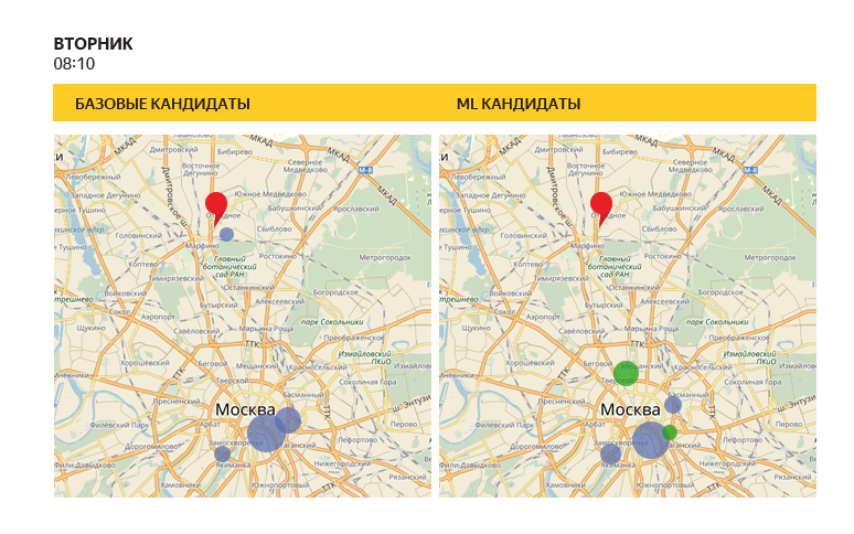
“Old” heuristics and a trained classifier can give different predictions: in this figure, the size of the circle shows how high this point is in the list of recommendations on a particular day and specific time. Please note that the trained algorithm in this example offered several additional locations (green circles).
Our task was to use the re-ranking of the most probable “points B” on top of the “old” strategy using machine learning. The general approach is this: first, we award points, as before, then we take the top n for these points (where n is obviously more than what we need to recommend), and then re-rank it and the user will only show the three most likely points B. Exact number The candidates in the list are, of course, determined in the course of optimization so that both the quality of candidates and the quality of re-ranking are as high as possible. In our case, the optimal number of candidates turned out to be 20.
About quality assessment and results
First, the quality must be divided into two parts: the quality of candidates and the quality of ranking. The quality of candidates is how well selected candidates are, in principle, correctly rearranged. And the quality of ranking is how well we predict the destination point, provided that it is among the candidates.
Let's start with the first metric, that is, the quality of candidates. It is worth noting that only about 72 percent of orders selected point B (or very close to it geographically) was present earlier in history. This means that the maximum quality of candidates is limited to this number, since we cannot yet recommend points to which a person has never traveled. We selected heuristics with assignment of points so that when selecting the top 20 candidates for these points the correct answer was contained in 71% of cases. With a maximum of 72%, this is a very good result. We were completely satisfied with this quality of candidates, so we didn’t touch this part of the model, although, in principle, we could. For example, instead of heuristics, it was possible to train a separate model. But since the heuristics-based search engine has already been technically implemented, we were able to save on development only by selecting the necessary coefficients.
Let's go back to the quality of re-ranking. Since we can show one, two, or a maximum of three points on the main screen of the trip order, we are interested in the proportion of cases when the correct answer was in the top-1, top-2 and top-3 ranking lists, respectively. In machine learning, the share of correct answers in the top k of the ranking list (of all correct answers) is called recall @ k. In our case, we are interested in recall @ 1, recall @ 2 and recall @ 3. In this case, the “correct answer” in our problem is only one (up to closely spaced points), which means that this metric will just show the proportion of cases when the real “point B” falls in the top 1, top 2 and top 3 of our algorithm .
As a basic ranking algorithm, we took the sort by the number of points and obtained the following results (in percent): recall @ 1 = 63.7; Recalling @ 2 = 78.5 and recall @ 3 = 84.6. Note that the percentages here are a fraction of those cases where the correct answer in the candidates was generally present . At some point a logical question arose: perhaps simple sorting by popularity already gives good quality, and all the ideas of sorting by points and using machine learning are superfluous? But no, such an algorithm showed the worst quality: recall @ 1 = 41.2; recall @ 2 = 64.6; recall @ 3 = 74.7.
Remember the original results and proceed to discuss the machine learning model.
The proportion of cases where the actual destination was among the first k recommendations
What model was built
To begin, we describe the mechanism for finding candidates. As we have already said, on the basis of statistics on user’s trips to different places, points are awarded. A point earns points if trips are made to or from it; and significantly more points get those points to which the user traveled from the place where he is now, and even more points if this happened around the same time. Further, the logic is clear.
We now turn to the model for re-ranking. Since we want to maximize recall @ k, in the first approximation we want to predict the likelihood of the user going to a certain place and rank the places by probability. “As a first approximation,” because these arguments are true only with a very accurate estimate of probabilities, and when errors appear in them, recall @ k can be better optimized by another solution. A simple analogy: in machine learning, if we know for sure all probability distributions, the best classifier is Bayesian , but since in practice distributions are reconstructed from data approximately, often other classifiers work better.
The classification task was posed as follows: the objects were couples (history of the user's previous trips; candidate for recommendations), where positive examples (class 1) were couples in which the user did go to this point B, negative examples (class 0) were pairs in which the user eventually went to another place.
Thus, if you were a hardened formalist, the model did not estimate the likelihood that a person would go to a specific point, but the shifted probability that a given “story-candidate” pair is relevant. However, sorting by this value is as meaningful as sorting by the probability of a trip to a point. It can be shown that with an excess of data, these will be equivalent sorts.
We trained the classifier to minimize log loss, and as a model, we used the Matrixnet actively used in Yandex (gradient boosting over decision trees). And if everything is clear with MatrixNet, then why was log loss optimized?
Well, first, the optimization of this metric leads to the correct estimates of probability. The reason why this happens is rooted in mathematical statistics, in the maximum likelihood method . Let the probability of a single class at the i-th object be pi and the true class is yi . Then, if we consider the outcomes independent, the likelihood of the sample (roughly speaking, the probability of obtaining exactly the outcome that was obtained) is equal to the following product:
prodipyii(1−pi)(1−yi)
Ideally, we would like to have such pi to get the maximum of this expression (because we want our results to be as credible as possible, right?). But if one prologicarizes this expression (since the logarithm is a monotonic function, then we can maximize it instead of the original expression), then we get sumiyiln(pi)+(1−yi)ln(1−pi) . And this is already known to us log loss, if you replace pi on their predictions and multiply the whole expression by minus one.
Secondly, we, of course, trust the theory, but just in case, we tried to optimize various loss functions, and the log loss showed the largest recall @ k, so everything eventually came together.
We talked about the method, the function of the error, too, one important detail remained: the signs by which we trained our classifier. We used more than a hundred different signs to describe each “history candidate” pair. Here are some examples:
And finally, about the results: after re-ranking using the model we built, we obtained the following data (again, in percent): recall @ 1 = 72.1 (+8.4); recall @ 2 = 82.6 (+4.1); recall @ 3 = 88 (+3,4). Not bad at all, but improvements are possible in the future due to the inclusion of additional information in the signs.
You can look at an example of how the new prediction algorithm will look to the user:
Future plans
Of course, there are many experiments to improve the model. There will be the addition of new data to build recommendations, including the interests of the user, as well as the alleged “home” and “work” from Yandex Crypt and related features, and an experiment comparing the various classification methods in this task. For example, Yandex already has not only used exclusively within the MatrixNet team, but also gaining popularity in Yandex and beyond its CatBoost . At the same time, of course, we are interested in comparing not only our own developments, but also other implementations of popular algorithms.
In addition, as already mentioned at the beginning of the post, it would be great if the application itself understood when, where, and on which car we needed to go. Now it’s hard to say how it is possible to accurately guess the order parameters and settings of the application suitable for the user from historical data, but we are working in this direction, we will make our application more “smart” and able to adapt to you.
Source: https://habr.com/ru/post/337328/
All Articles