Hello! My name is Kirill and I have been an alcoholic for more than 10 years as an IT manager. I was not always like this: while studying at MIPT, I wrote a code, sometimes for a reward. But faced with the harsh reality (in which you need to make money, preferably more), he went downhill - in managers.

But it is not all that bad! Recently, we and our partners have completely and completely gone into the development of their startup: the accounting system for customers and customer requests Okdesk . On the one hand - more freedom in choosing the direction of movement. But on the other hand, it’s impossible to simply take and pledge the budget of "3 developers for 6 months for research and development of a prototype for ...". You have to do a lot yourself. Including - non-core experiments associated with the development (ie, those experiments that do not relate to the main functionality of the product).

One of such experiments was the development of an algorithm for classifying client requests by texts for further routing to a group of performers. In this article I want to tell you how a “non-programmer” can master python in the background for 1.5 months in the background and write a simple ML algorithm that has practical utility.

How to study?

In my case - distance learning on Coursera. There are quite a few courses in machine learning and other disciplines related to artificial intelligence. Classics is the course course founder Andrew Una (Andrew Ng). But the disadvantage of this course (besides the fact that the course is in English: this is not for everyone) is a rare Octave toolkit (a free analogue of MATLAB). To understand the algorithms is not important, but it is better to learn from the more popular tools.
')
I chose the specialization " Machine learning and data analysis " from MIPT and Yandex (there are 6 courses in it; the first 2 are enough for what is written in the article). The main advantage of specialization is a vibrant community of students and mentors in Slack, where almost every time there is someone you can contact with a question.

What is Machine Learning?

Within the framework of the article we will not dive into terminological disputes, therefore, those who want to find fault with insufficient mathematical accuracy, please refrain (I promise that I will not go beyond the bounds of decency :).

So what is machine learning? This is a set of methods for solving problems that require any intellectual expenditure of a person, but with the help of computers. A characteristic feature of machine learning methods is that they “learn” from precedents (that is, from examples with known correct answers in advance).

A more mathematically defined definition looks like this:

1. There are many objects with a set of characteristics. Denote this set by the letter X ;
2. There are many answers. Denote this set by the letter Y ;
3. There is a (unknown) relationship between the set of objects and the set of answers. Those. such a function that associates an object of a set X with an object of a set Y. Let's call it a function y ;
4. There is a finite subset of objects from X (training sample) for which the answers from Y are known;
5. According to the training sample, it is necessary to approximate the function y as well as possible with some function a . With the help of the function a, we want for any object from X to get with a good probability (or accuracy - if we are talking about numerical answers) the correct answer from Y. The search for the function a is a machine learning task.

Here is an example from life. Bank grants loans. The bank has accumulated a lot of borrower questionnaires for which the outcome is already known: they returned the loan, did not return it, returned it in arrears, etc. The object in this example is the borrower with a completed application form. Data from the questionnaire - the parameters of the object. The fact of repayment or non-repayment of the loan is the "answer" on the object (the borrower's questionnaire). The set of questionnaires with known outcomes is a training sample.

There is a natural desire to be able to predict the repayment or non-repayment of a loan by a potential borrower on his profile. The search for a prediction algorithm is a machine learning task.

There are many examples of machine learning tasks. In this article we will talk more about the task of classifying texts.

Formulation of the problem

Recall that we are developing Okdesk - a cloud service for customer service. Companies that use Okdesk in their work accept client applications via different channels: client portal, email, web forms from the site, instant messengers, and so on. The application may fall into one category or another. Depending on the category, the application may have one or another performer. For example, applications for 1C should be sent to a decision to 1C specialists, and applications related to the work of an office network should be sent to a group of system administrators.

To classify the flow of requests, you can select the dispatcher. But, first, it costs money (salary, taxes, office rent). And secondly, time will be spent on the classification and routing of the application and the application will be solved later. If you could classify an application by its content automatically - it would be great! Let's try to solve this problem by machine learning (and one IT manager).

For the experiment, a sample of 1200 applications was taken with affixed categories. In the sample, applications are divided into 14 categories. The purpose of the experiment: to develop a mechanism for automatic classification of applications according to their content, which will give several times better quality than random. According to the results of the experiment, it is necessary to make a decision on the development of the algorithm and the development of an industrial service on its basis for the classification of applications.

Tools

The experiment was carried out using a Lenovo laptop (core i7, 8GB of RAM), the Python 2.7 programming language with the NumPy, Pandas, Scikit-learn, re libraries and the IPython shell. I will write more about libraries used:

1. NumPy is a library containing a variety of useful methods and classes for conducting arithmetic operations with large multidimensional numeric arrays;
2. Pandas is a library that allows you to easily and easily analyze and visualize data and conduct operations on them. The main data structures (object types) are the Series (one-dimensional structure) and the DataFrame (two-dimensional structure; in fact, the Series is of the same length).
3. Scikit-learn is a library that implements most of the methods of machine learning;
4. Re - library of regular expressions. Regular expressions are an indispensable tool in tasks related to text analysis.

From the Scikit-learn library, we will need some modules, the purpose of which I will write in the course of the presentation of the material. So, we import all the necessary libraries and modules:

import pandas as pd import numpy as np import re from sklearn import neighbors, model_selection, ensemble from sklearn.grid_search import GridSearchCV from sklearn.metrics import accuracy_score 

And we proceed to the preparation of data.

(the construction import xxx as yy means that we include the xxx library, but in the code we will access it through yy)

Data preparation

When solving the first real (and not laboratory) tasks related to machine learning, you will discover that most of the time is spent not on learning the algorithm (choosing an algorithm, selecting parameters, comparing the quality of different algorithms, etc.). The lion's share of resources will be spent on collecting, analyzing and preparing data.

There are various techniques, methods, and recommendations for preparing data for different classes of machine learning tasks. But most experts call data preparation art rather than science. There is even such an expression - feature engineering (i.e., construction of parameters describing objects).

In the task of classifying texts, the object has one text - text. You cannot feed it to the machine learning algorithm (I admit that I do not know everything :). The text needs to be digitized and formalized.

As part of the experiment, primitive methods of text formalization were used (but even they showed a good result). We will discuss this further.

Data loading

Recall that as the source data we have unloading 1200 applications (distributed unevenly in 14 categories). For each application there is a "Subject" field, a "Description" field and a "Category" field. The "Subject" field is the abbreviated content of the application and it is mandatory, the "Description" field is an extended description and it may be empty.

The data is loaded from the .xlsx file into the DataFrame. There are a lot of columns in the .xlsx file (parameters of real requests), but we need only the "Subject", "Description" and "Category".

After downloading the data, we combine the "Subject" and "Description" fields into one field for the convenience of further processing. To do this, you must first fill in all the empty Description fields (with an empty string, for example).

 #   issues  DataFrame issues = pd.DataFrame() #   issues  Theme, Description  Cat,     ,     .xlsx . u'...' —   '…'  utf issues[['Theme', 'Description','Cat']] = pd.read_excel('issues.xlsx')[[u'', u'', u'']] #     Description   issues.Description.fillna('', inplace = True) #   Theme  Description (    )   Content issues['Content'] = issues.Theme + ' ' + issues.Description 

So, we have a variable of DataFrame type, in which we will work with the columns Content (combined field for the "Subject" and "Description" fields) and Cat (category of the application). Let us proceed to the formalization of the content of the application (ie, the Content column).

Formalization of the content of applications

Description of the approach to formalization

As mentioned above, the first step is to formalize the text of the application. The formalization will be carried out as follows:

1. We divide the content of the application into words. By a word we mean a sequence of 2 or more characters, separated by delimiting characters (dashes, hyphens, full stops, spaces, new lines, etc.). As a result, for each application we get an array of words contained in its content.
2. From each application, we exclude “parasite words” that do not carry meaning (for example, words included in greeting phrases: “hello”, “good”, “day”, etc.);
3. From the resulting arrays we compose a dictionary: a set of words used to write the content of all applications;
4. Next, we compose a matrix of size (number of applications) x (the number of words in the dictionary) , in which the i-th cell in the j-th column corresponds to the number of entries in the i-th application of the j-th word from the dictionary.

The matrix of paragraph 4 is a formalized description of the content of applications. Speaking in a mathematized language, each row of the matrix is ​​the coordinates of the vector of the corresponding application in the dictionary space. For learning the algorithm, we will use the resulting matrix.

Important point : p.3 is carried out after we select a random subsample from the training sample for the quality control of the algorithm (test sample). This is necessary in order to better understand what quality the algorithm will show "in battle" on new data (for example, it is not difficult to implement an algorithm that will give ideally correct answers on the training set, but random data will not work better on any new data : this situation is called retraining). The separation of the test sample before the compilation of the dictionary is important because if we had compiled a dictionary including on the test data, then the algorithm trained on the sample would turn out to be already familiar with unknown objects. Conclusions about its quality on unknown data will be incorrect.

Now we will show how p.p. 1-4 look in the code.

We break the content into words and remove the word parasites

First of all, we will bring all the texts to lower case (“printer” and “Printer” are the same words only for a person, not for a machine):

 #       def lower(str): return str.lower() #      Content issues['Content'] = issues.Content.apply(lower) 

Next, we define an auxiliary dictionary of “words-parasites” (its content was made by experimentally iteratively for a specific sample of applications):

 garbagelist = [u'', u'', u'', u'', u'',u'', u'', u'', u''] 

We declare a function that splits the text of each application into words of 2 or more characters and then includes the words obtained, with the exception of “parasite words”, into an array:

 def splitstring(str): words = [] #     [] for i in re.split('[;,.,\n,\s,:,-,+,(,),=,/,«,»,@,\d,!,?,"]',str): #  ""  2    if len(i) > 1: #  - if i in garbagelist: None else: words.append(i) return words 

For splitting text into words into separator characters, the re regular expression library and its split method are used. The split method is passed an array of delimiter characters (the delimiter character set is replenished iteratively and experimentally) and the string to be split.

We apply the declared function to each application. At the output, we obtain the original DataFrame, in which a new column appeared, Words with an array of words (with the exception of “parasite words”), of which each application consists.

 issues['Words'] = issues.Content.apply(splitstring) 

Compiling a dictionary

Now we will start to compile a dictionary of words included in the content of all applications. But before this, as was written above, we divide the training sample into a control one (also known as “test”, “delayed”) and the one on which we will train the algorithm.

The sampling is carried out using the train_test_split method of the model model module_selection of the Scikit-learn library. In the method we pass an array with data (application texts), an array with labels (categories of applications) and a test sample size (usually 30% of the total is selected). At the output we get 4 objects: data for training, tags for training, data for control and tags for control:

 issues_train, issues_test, labels_train, labels_test = model_selection.train_test_split(issues.Words, issues.Cat, test_size = 0.3) 

Now we will declare a function that will make a dictionary of the data left for training ( issues_train ), and apply the function in this data:

 def WordsDic(dataset): WD = [] for i in dataset.index: for j in xrange(len(dataset[i])): if dataset[i][j] in WD: None else: WD.append(dataset[i][j]) return WD #    words = WordsDic(issues_train) 

So, we have compiled a dictionary of words that make up the texts of all applications from the training set (with the exception of applications left under control). The dictionary was recorded in the variable words. The size of the array of words turned out to be 12015th elements (i.e. words).

We translate the content of applications into the dictionary space

We proceed to the final step of preparing data for training. Namely: we compose a matrix of size (number of applications in the sample) x (the number of words in the dictionary) , where the i-th row of the j-th column contains the number of occurrences of the j-th word from the dictionary in the i-th request from the sample.

 #   len(issues_train)  len(words),    train_matrix = np.zeros((len(issues_train),len(words))) # ,   [i][j]   j-   words  i-    for i in xrange(train_matrix.shape[0]): for j in issues_train[issues_train.index[i]]: if j in words: train_matrix[i][words.index(j)]+=1 

Now we have everything necessary for learning: the train_matrix matrix (the formalized content of applications in the form of coordinates of vectors, corresponding to applications, in the dictionary space compiled for all applications) and labels_train labels (categories of applications from the sample left for training).

Training

We now turn to learning algorithms on tagged data (that is, data for which the correct answers are known: the train_matrix matrix with labels labels_train ). In this section there will be little code, since most of the methods of machine learning are implemented in the Scikit-learn library. Developing your own methods can be useful for mastering the material, but from a practical point of view there is no need for this.

Below I will try to explain in simple language the principles of specific methods of machine learning.

On the principles of choosing the best algorithm

You never know which machine learning algorithm will give the best result on specific data. But, understanding the task, you can determine the set of the most appropriate algorithms so as not to go through all the existing ones. The choice of the machine learning algorithm that will be used to solve the problem is carried out through a comparison of the quality of the algorithms on the training set.

What counts as the quality of the algorithm depends on the task you are solving. The choice of quality metrics is a separate large topic. As part of the classification of applications, a simple metric was chosen: accuracy (accuracy). Accuracy is defined as the proportion of objects in the sample for which the algorithm gave the correct answer (set the correct category of the application). Thus, we will choose the algorithm that will give greater accuracy in predicting the categories of applications.

It is important to say about such a concept as the hyperparameter of the algorithm. Machine learning algorithms have external (ie, those that cannot be derived analytically from a training set) parameters that determine the quality of their work. For example, in algorithms where you need to calculate the distance between objects, distance can be understood as different things: the Manhattan distance , the classical Euclidean metric , etc.

Each machine learning algorithm has its own set of hyperparameters. The choice of the best values ​​of the hyperparameters is carried out, oddly enough, by an exhaustive search: the quality of the algorithm is calculated for each combination of parameter values ​​and then the best combination of values ​​is used for this algorithm. The process is costly in terms of computing, but where to go.

Cross-validation is used to determine the quality of the algorithm for each combination of hyperparameters. I will explain what it is. The training set is divided into N equal parts. The algorithm is sequentially trained on a subsample of N-1 parts, and the quality is considered to be one delayed. As a result, each of the N parts is used 1 time to calculate the quality and N-1 time to train the algorithm. The quality of the algorithm on the combination of parameters is calculated as the average between the quality values ​​obtained during cross-validation. Cross-validation is necessary in order for us to trust the obtained quality value more (by averaging, we level possible “distortions” of a particular sample break). A little more you know where .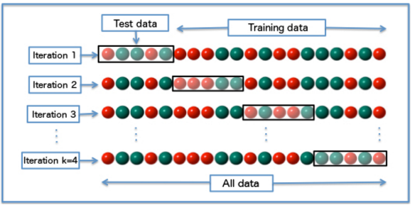



So, to choose the best algorithm for each algorithm:

1. All possible combinations of hyperparameter values ​​are searched (each algorithm has its own set of hyperparameters and their values);
2. For each combination of hyperparameter values ​​using cross-validation, the quality of the algorithm is calculated;
3. The algorithm is selected with the combination of values ​​of the hyperparameters, which shows the best quality.

From the point of view of programming of the algorithm described above, there is nothing complicated. But in this there is no need. In the Scikit-learn library there is a ready-made method for selecting parameters according to the grid (the GridSearchCV method of the grid_search module). All that is needed is to transfer the algorithm, the parameter grid and the number N to the method (the number of parts into which we divide the sample for cross-validation; they are also called "folds").

In the framework of solving the problem, 2 algorithms were chosen: k nearest neighbors and the composition of random trees. About each of them the story further.

k nearest neighbors (kNN)

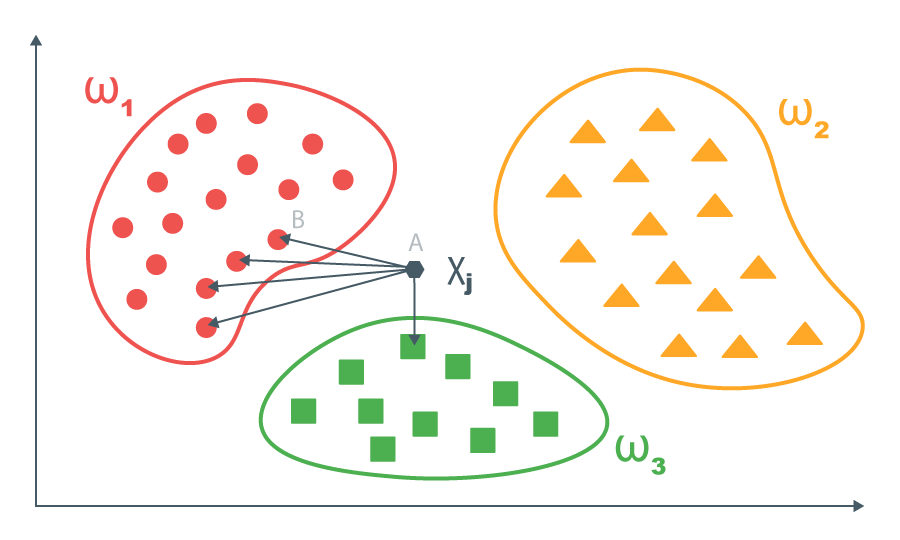
The k-nearest-neighbor method is the easiest to understand. It consists in the following.

There is a training set, the data in which are already formalized (prepared for training). That is, objects are represented as vectors of some space. In our case, applications are presented in the form of vectors of the dictionary space. For each vector of the training set, the correct answer is known.

For each new object, pairwise distances between this object and the objects of the training sample are calculated. Then, the k nearest objects are taken from the training set, and for the new object, the answer that prevails in the subsample of k nearest objects is returned (for tasks where you need to predict the number, you can take the average value of the k closest ones).

The algorithm can be developed: to give more weight to the value of the label on a closer object. But for the task of classifying applications we will not do this.

In our problem, the hyperparameters of the algorithm are the number k (since our nearest neighbors will draw a conclusion) and the determination of the distance. The number of neighbors is enumerated in the range from 1 to 7, the determination of the distance is chosen from the Manhattan distance (the sum of the modules of the coordinate difference) and the Euclidean metric (the root of the sum of the squares of the coordinate difference).

We execute a simple code:

 %%time #     param_grid = {'n_neighbors': np.arange(1,8), 'p': [1,2]} #  fold-  - cv = 3 #  estimator_kNN = neighbors.KNeighborsClassifier() # ,    fold-       optimazer_kNN = GridSearchCV(estimator_kNN, param_grid, cv = cv) #        optimazer_kNN.fit(train_matrix, labels_train) #         print optimazer_kNN.best_score_ print optimazer_kNN.best_params_ 

After 2 minutes and 40 seconds, we learn that the best quality at 53.23% shows the algorithm on the 3 nearest neighbors, determined from the Manhattan distance.

Arrangement of random trees

Decisive trees

Decisive trees are another machine learning algorithm. The learning algorithm is a step-by-step partition of the training sample into parts (most often into two, but in general it is not necessary) according to some feature. Here is a simple example illustrating the work of the decision tree:

The decision tree has internal vertices (at which decisions are made on the further partitioning of the sample) and final vertices (sheets), which are used to predict the objects that went there.

In the decision vertex, a simple condition is checked: the conformity of some (about this later) j object attribute to the condition x ^{j is} greater than or equal to some t. Objects that satisfy the condition are sent to one branch, and not satisfying - to another.

When learning the algorithm, it would be possible to split the training sample until all the nodes have one object at a time. This approach will give an excellent result on the training sample, but on the unknown data you will get a “hat”. Therefore, it is important to define the so-called “stopping criterion” - the condition under which the vertex becomes a leaf and the further branching of this vertex stops. The stopping criterion depends on the task, here are some types of criteria: the minimum number of objects at the vertex and the limit on the depth of the tree. In solving the problem, we used the criterion of the minimum number of objects at the vertex. A number equal to the minimum number of objects is an algorithm hyperparameter.

New (requiring prediction) objects are driven along a trained tree and fall into the corresponding sheet. For objects on the list, we give the following answer:

1. For classification tasks, we return the most common class of objects of the training set in this sheet;
2. For regression tasks (i.e., those where the answer is a number) we return the average value on the objects of the training sample from this sheet.

It remains to talk about how to select for each vertex the attribute j (according to which criterion we divide the sample at a particular vertex of the tree) and the threshold t corresponding to this attribute. For this purpose, the so-called error criterion Q (X _m , j, t) is introduced. As you can see, the error criterion depends on the sample X _m (that part of the training sample that reached the vertex under consideration), the parameter j, which will be used to split the sample X _m in the vertex under consideration and the threshold value t. It is necessary to choose j and t such that the error criterion will be minimal. Since the possible set of values ​​of j and t for each training sample is limited, the problem is solved by enumeration.

What is the error criterion? The draft version of the article on this site contained many formulas and accompanying explanations, a story about the informativeness criterion and its particular cases (the Ginny criterion and the entropy criterion). But the article turned out and so bloated. Those who want to understand the formalities and mathematics can read about everything on the Internet (for example, here ). Limited to the "physical meaning" on the fingers. The error criterion shows the level of "diversity" of objects in the resulting subsamples. By "diversity" in classification problems we mean a variety of classes, and in regression problems (where we predict numbers), dispersion. Thus, when dividing the sample, we want to maximally reduce the “diversity” in the resulting subsamples.

With trees sorted out. We turn to the composition of trees.

The composition of the decisive trees

Decisive trees can reveal very complex patterns in the training set. , — . ().

N “”. (, ) , — ( N ) .

, N . : N . : / (.. , ). — (.. , ; , — ). .

- ! 2- : ( ) ( ).

:

 %%time #     param_grid = {'n_estimators': np.arange(20,101,10), 'min_samples_split': np.arange(4,11, 1)} #  fold-  - cv = 3 #  estimator_tree = ensemble.RandomForestClassifier() # ,    fold-       optimazer_tree = GridSearchCV(estimator_tree, param_grid, cv = cv) #        optimazer_tree.fit(train_matrix, labels_train) #         print optimazer_tree.best_score_ print optimazer_tree.best_params_ 

3 30 , 65,82% 60 , 4.

Result

(, — ) .

test_matrix, , (.. , train_matrix, ).

 #   len(issues_test)  len(words) test_matrix = np.zeros((len(issues_test),len(words))) # ,   [i][j]   j-   words  i-    for i in xrange(test_matrix.shape[0]): for j in issues_test[issues_test.index[i]]: if j in words: test_matrix[i][words.index(j)]+=1 

accuracy_score metrics Scikit-learn. :

 print u' :', accuracy_score(optimazer_tree.best_estimator_.predict(test_matrix), labels_test) print u'kNN:', accuracy_score(optimazer_kNN.best_estimator_.predict(test_matrix), labels_test) 

51,39% k 73,46% .

""

, “ ” , random. “” , random. , “” , - .

3- “” :

1. random;
2. ;
3. Random, .

random 14 100/14 * 100% = 7,14% . , 14,5% ( ). random- . , random-:

 #  random import random # ,    random-  rand_ans = [] # for i in xrange(test_matrix.shape[0]): rand_ans.append(labels_train[labels_train.index[random.randint(0,len(labels_train))]]) #  print u' random:', accuracy_score(rand_ans, labels_test) 

14,52%.

, , “” . Hooray!

What's next?

, 90% — . , . “” ( , ). -, (: " ", " ", " " ..) — ( ) .

, : . " " "", . . , , , .

, Okdesk .

"! !" (with)

( 2). .