“Rise of Machinery Learning” or combine a hobby in Data Science and analyzing the spectra of light bulbs
In the final article of the cycle devoted to the study of Data Science from scratch , I shared my plans to combine my old and new hobby and place the result on Habré. Since past articles have found a lively response from readers, I decided not to postpone it for long.
So, for the past several years I have been busy in my spare time in questions related to lighting and most of all I am interested in the spectra of various light sources, like “ancestors” of the characteristics derived from them. But not so long ago, I accidentally had another hobby - machine learning and data analysis, in this matter I am an absolute beginner, and in order to have fun, I periodically share my newfound experience and stuffed "bumps"
This article is written in the style of newbies to beginners , so experienced readers are unlikely to get something new for themselves, and if there is a desire to solve the problem of classifying light sources according to spectra, then it makes sense to immediately get data from GitHub
')
And for those who do not have a great experience, I will suggest continuing our joint training and this time try to take up the task of machine learning, which is called “for yourself”.
We will go with you from trying to understand where you can apply even a little knowledge of ML (which can be obtained from basic books and courses), to solving the very task of classification itself and thinking about "what to do now with all this ?!"
You are welcome all under the cat.

So, colleagues in front of us is a very important mission to find out how dangerous artificial intelligence is, is it time for us to blow up Skynet or can we spend a little more time watching videos with cats.
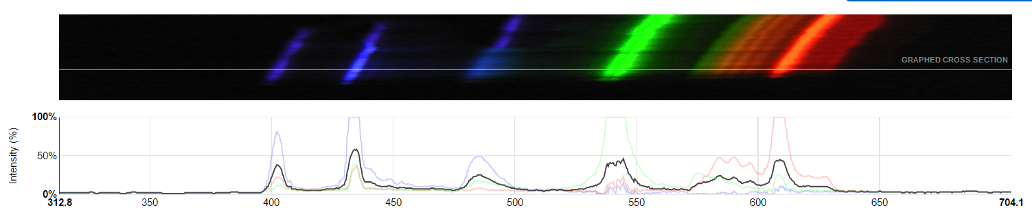
In this article, we will, on the basis of approximately such images, determine what type of lamp the lamp is in: fluorescent or LED, or perhaps even the light of the sun and sky.
Let's start with a rather important point , namely with the requirements for skills. As in the previous articles, I share with you the experience that I managed to get myself and before starting the article it is important to understand that it can be useful to people with similar experiences. As I said earlier, material is unlikely to be useful to experienced specialists.
Although they can certainly find some mistakes in it and tell me about it, so that I can correct them if possible.
This time, in order for the article not to cause you difficulties, we already need some basic skills, namely:
If you have taken online courses or have read a self-instruction manual, I think this will be quite enough.
The second important point to understand why we all do it?
Indeed, if you just want to practice analyzing data and solving machine learning problems, then there are many wonderful tasks on Kagle, including those suitable for absolute beginners (for example, about Titanic).
Most likely, these tasks will be more correct and in cases with tasks for beginners you will surely find more successful tutorials than in our case, so if you still do not itch your hands to “invent your own bike” or do not have enough skills, then it makes sense to practice Kagle ( I wrote about this before ).
In the book Data Science from Scratch , closer to the end, the author suggested not dwelling on the materials of the book and coming up with a task on my own, while sharing my ideas, at that moment I thought: “Of course, you are so smart, but I have no idea what to do! ".
In my opinion, this idea was very fair, because it is hard to learn from this book, something very useful in practice ( for more details on this in the review ). And in the end, before sculpting dumplings, it probably makes sense to try them all the same, and it is advisable to try the good ones, so that is what it seeks.
In the Specialization "Machine Learning and Data Analysis", through the eyes of a newbie in Data Science "on Coursera ( review ), there was something to try and get a hand on what, and after passing it, it became certain that now it’s not perfect, but You can collect and analyze data yourself.
Summing up the chapter, I want to say, from a pedagogical point of view, I consider VERY useful and important the stage of self-setting the problem for machine learning, even if it is purely “fake”. That is why I decided to share my example with you.
Let's address the question of where to get the material (data) for our research.
In my opinion, the source itself is not so important, the main thing is that the subject matter is close to you and you can find more or less a sufficient amount of reliable data.
Well, for example:
1. You can classify your friends by text messages in the social. networks (someone is silent, someone often uses keywords, someone puts a bunch of emoticons, and so on)
2. Or, based on past data (well, for example, utility bills), you can predict how much hot water or electricity you will spend this November.
3. And you can restore the relationship between the rating of the downloaded series and the number of "snacks" that you eat when viewing it.
4. If you are a very angry person, try to solve the problem of the number of cats in your single friends
5. If you have a hard time with personal experience and you do not store archives in yellowed folders, look at the domestic (or foreign) open data portals data.gov.ru or for Moscow data.mos.ru , for example, you can find the data in order to predict the number of calls of firefighters in a particular district of Moscow in the future, and then check in a couple of months.
In our case, I did not need to go far for data. There is a wonderful opensource project Public Lab, in which there is a subsection devoted to the analysis of the spectrum of light sources .
Two words about him:
The project proposes to assemble a spectroscope from available tools ( well, for example, from cardboard and DVD discs ) and photograph the spectra.
After you take a bunch of spectra images, it would be good to study them in more detail. To do this, they have a web interface on the site that allows you to load and process your spectrum a bit to get a digital view of it (for example, as a table). .
All data is in the public domain, anyone can either download the spectrum to the portal or download data. This openness has one big flaw, which we will need to take into account, but about it a little later (just decided to introduce intrigue into the story) .
There are many pictures on the portal, though it’s important to remember that among the pictures you don’t have to be the spectra of light bulbs, for example, there can be light reflectance spectra of materials or light transmission spectra of various liquids.
In any case, we have visual open data that are unified, structured and most importantly can be downloaded in a convenient format (for example, .csv), what else can you dream of?
(except a million dollars and a personal helicopter)
Consider the data that we have and what we want to get in the end.
Hereinafter I will focus on the files in the format csv
So we have the distribution of radiation power (conditional) along the wavelength of the spectrum ( spectral distribution of radiation density ).
In the data downloaded from the Public Lab there is an average value as well as broken down by the R, G, B channels, we will only be worried about the average.
If you just simplify the description, then when passing through a diffraction grating or prism, the light splits into a rainbow, and if sunlight gives you a rainbow, as in the saying about the pheasant, then the light of poor-quality fluorescent lamps may look like a hockey player Ovechkin’s smile (certainly charming, but with some spaces) .
It is precisely on the basis of this structure of the rainbow that we will classify the spectra.
Since all algorithms and libraries for machine learning are written by living people (for the time being), in many respects they are a formalization of those things that we often do unconsciously when solving certain tasks.
On the one hand, the data set that I have compiled for you is very simple - the classes are balanced, the signs have a more or less close scale, there are no obvious emissions, so some things that they write in the training materials I cannot demonstrate to you on it.
On the other hand, who knows, maybe we are all robots? Therefore, I will cover a couple of points that would be important to note, as if we had written a model for collecting data instead of doing it manually.
To begin, let us recall the important points that are often talked about and written in educational materials:
Knowledge of the specifics
In the training materials they write that for machine learning it is important to have knowledge of the field of activity for which we are preparing the model. And with this I fully agree, it is not enough to know all the algorithms and methods, to be able to use libraries. Ignorance of some nuances can cover your model with a copper basin and reduce its value to zero.
Let's turn to our case. Remember I talked about the BIG minus of the openness of the platform (with all its advantages). So, people can pour in any photographs of the spectra taken on instruments of any quality, and then process them as they will enter the head.
The most important point to consider is the correct calibration of the spectrum.
The mechanism is as follows: you photograph a characteristic object (a compact fluorescent lamp) and on the basis of it you get a scale of your distribution (based on two peaks of blue and green).
It doesn’t sound very difficult, but you need to tamper a little, firstly, not everyone speaks English, and secondly, not everyone likes to read the instructions, therefore, even now the mechanism has been simplified (by adding a sample), but there is still a risk stumble on an improperly calibrated spectra. In the end, the spectra can be loaded by children and some of them can be hard to figure out on their own.
Therefore, on the one hand, we have a lot of simply uncalibrated images, on the other hand, a certain amount of incorrectly calibrated ones, which is much worse.
For example, there is a photo under it there is a graph like something more or less meaningful (without noise), but naturally this is an incorrect calibration (turquoise should be around 500 nm, and orange around 600 nm.)

This is not the worst example, there are cases where poor calibration is present, but it is much less striking, but I just did not find them without thinking.
The second point is that we don’t really know which spectra (which lamps), under what conditions and what the users photographed them, so at least it’s important to know that you shouldn’t trust the data to 100%. Sometimes some spectra are suspicious.
The third point, it is important to remember about the technical limitations, in most cases, this measuring circuit strongly cuts spectra in the red range of light, therefore, for example, data beyond 600 nm. may not be less reliable and not the fact that they will correspond to the true spectra. The situation is similar with violet (ultraviolet) light.
The fourth point, part of the radiation in the spectra can be cut off, due to the high brightness of the images, this distorts the data and sometimes it can also be important. Maybe there are some other nuances that I did not remember or do not know. So, without knowing even these trifles, it would be possible to make mistakes when preparing the samples.
Signs and data selection
Regarding the signs, let the radiation power for each wavelength be our feature for the future model.
Considering the above, it becomes clear that for classifying us there is not much point in taking the spectrum, in the range that the system gives (sometimes almost from 200 to 1000 nm), take the range from 390 to 690 even this is a bit redundant (because everywhere there is this data), but we don’t seem to lose anything significant.
We divide the signs in steps of 1 nm. Well, for example, 400, 401, 402 ... It would be possible to take a step less often, for example, 10 nm., but we will have a small sample and even 301 signs will not overload our computer when calculating. In theory, increasing the pitch reduces the accuracy of the model, but also drastically reduces the pitch, for example, to 0.25 nm. we do not much weather, and machine resources will eat.
Concerning the selection of spectra
Initially I wanted to make a larger sample with a large number of classes, but it stalled, as I said before, not all spectral images could be used due to poor calibration, noise, or doubts about the reliability.
Therefore, in the end, we limit ourselves to three classes: daylight (sky, sun or all together), fluorescent lamps (both compact and tubular), and LED lamps (white with phosphor and based on RGB LEDs).
I hope that everything that I have gathered to you is shining with white light (of various shades and of different quality).
When collecting data, the problem with poor data calibration for fluorescent lamps was easy to solve; it was enough to calibrate them yourself. But with daylight and LED lamps such a trick will not work (there is often a smooth spectrum), well, at that time I did not find incandescent lamps (calibrated) in sufficient quantities, but new data are actively added there if you consider it necessary to expand the sample and make the task more interesting.
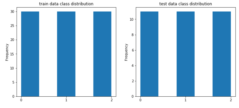
To make it easier to classify as a result, I made the sample uniform. In the training set of 30 records of each class, in the control sample of 11 records.
And even though I was a little tired and confused at the end, the sample should contain examples of different light sources, different lamps, different LEDs, etc.
In this case, I combed the sample for you, but in a real sample, you may have to process the data yourself.
Another point about the sample.
There is such a thing in statistics as errors of the first kind and second kind. In a very simplified presentation: you hypothesize that there is paper in the toilet, which means you don’t take it with you, so if in this situation you insure and take a roll with you in vain (a false positive is a mistake of the first kind), then not as scary as if you don’t grab a roll, and there will only be a cardboard ring (a mistake of the second kind).
So, when choosing data, I tried to minimize the error of the second kind, it was not very scary for us to skip the normal spectrum, but accidentally taking an erroneous spectrum into the sample is clearly not what we need.
But when solving the classification problem directly, any of the errors does not have a higher priority; when it is solved directly by the model, it is important for us that everything is absolutely predicted correctly and without reinsurance.
This is what determines the sufficiency of the metrics accuracy.
Well, there was a lot of text, let's finally move on closer to the model.
At https://github.com/bosonbeard/ML_light_sources_classification/tree/master/1st_spectrum_classification located:
I mean that you already have basic knowledge and you will have enough of them to understand my code far from the reference.
Import libraries:
Read the data:
In this case, we use the pandas library and its dataframe class, which, to put it simply, gives us the functions that Excel would give, that is, work with tables.
As I said earlier, in table 391 the column corresponds to the radiation power by wavelength, and the last column is the class label: 0 - LED, 1 - lum. lamps. 2 - daylight.
For further work, we immediately cut out 391 columns with signs and the last columns with labels into separate variables.
In normal work, a decent analysis of the initial data usually goes on, but we have nothing to analyze, as I said, all classes are balanced and, in principle, do not need much additional scaling (although you can scale it out of curiosity).
For the sake of form, I derived 2 graphics, if you want you can do something else.
Classification
Let's build our first model. Take one of the most popular models - the random forest model (decisive trees).
Let's see the results.
(predicted, actual):
(2, 0), (0, 0), (0, 0), (0, 0), (0, 0), (0, 0), (1, 0), (0, 0), (2 , 0), (2, 0), (2, 0), (1, 1), (1, 1), (1, 1), (1, 1), (0, 1), (1, 1 ), (1, 1), (1, 1), (1, 1), (1, 1), (1, 1), (2, 2), (2, 2), (2, 2), (2, 2), (2, 2), (2, 2), (2, 2), (2, 2), (2, 2), (2, 2), (2, 2)
Accuracy prediction (share of correct answers) = 0.8181818181818182
It turns out we can hope that our model will be 8 out of 10 spectra correctly classified, which is already good.
For the demonstration, we specifically took the best parameters for this model, let's try to sort through models with different parameters and select the best one based on the results of cross-checking.
We get the following parameters:
{'max_depth': 6, 'n_estimators': 30} 0.766666666667
best accuracy on cv: 0.77
accuracy on test data: 0.87879
best params: {'max_depth': 6, 'n_estimators': 30}
(predicted, actual):
[(0, 0), (0, 0), (0, 0), (0, 0), (0, 0), (0, 0), (0, 0), (0, 0), ( 2, 0), (2, 0), (2, 0), (1, 1), (1, 1), (1, 1), (1, 1), (0, 1), (1, 1), (1, 1), (1, 1), (1, 1), (1, 1), (1, 1), (2, 2), (2, 2), (2, 2) , (2, 2), (2, 2), (2, 2), (2, 2), (2, 2), (2, 2), (2, 2), (2, 2)]
Wall time: 1min 6s
That is, an increase of max_depth by 1 improves accuracy by 6%, which is not bad, despite the fact that the model with the number of trees (n_estimators), like “you will not spoil the porridge with oil,” the model decided that it is not worth further increasing their number (this saves resources).
I think you can achieve better results if you search for more parameters (or increase the sample size), but in order to demonstrate that the calculation does not take much time, we will limit ourselves to what it is.
So, you and I can start with our more advanced T-1000, so let's try to force something to classify our “Iron Arnie” as a simpler Logistic Regression model.
As one would expect, the simpler model from the first approach gave a little worse result.
results (predict, real):
[(0, 0), (0, 0), (0, 0), (2, 0), (0, 0), (0, 0), (0, 0), (2, 0), ( 0, 0), (0, 0), (2, 0), (1, 1), (1, 1), (1, 1), (1, 1), (2, 1), (2, 1), (1, 1), (1, 1), (1, 1), (1, 1), (2, 1), (2, 2), (2, 2), (2, 2) , (0, 2), (2, 2), (2, 2), (2, 2), (2, 2), (2, 2), (2, 2), (2, 2)]
accuracy score = 0.7878787878787878
We can play again with the parameters:
Results:
best accuracy on cv: 0.79
accuracy on test data: 0.81818
best params: {'C': 0.02, 'penalty': 'l1'}
(predicted, actual):
[(0, 0), (0, 0), (0, 0), (2, 0), (0, 0), (0, 0), (0, 0), (0, 0), ( 0, 0), (0, 0), (2, 0), (1, 1), (1, 1), (1, 1), (1, 1), (2, 1), (2, 1), (1, 1), (1, 1), (1, 1), (1, 1), (2, 1), (2, 2), (2, 2), (2, 2) , (0, 2), (2, 2), (2, 2), (2, 2), (2, 2), (2, 2), (2, 2), (2, 2)]
Wall time: 718 ms
So, we have achieved a quality comparable to Random forest without fitting the parameters, but we have spent significantly less time. It is seen precisely for this reason in the books they write that logistic regression is often used at the preliminary stages, when it is important to identify general patterns, and 5-7% of the weather will not be done right away.
On the one hand, this could be the end, but let's also try to imagine that I, as a dishonest person, gave you data without any description and you need to try to understand something without having class marks.
Clustering
For clarity, let's set the colors. I'm still a little cunning, in an amicable way, “we don’t know” that we have no more than three classes, but we really do know that, so we’ll confine ourselves to three colors.
To begin with, we will try to look at our data, we have almost 400 signs and on the two-dimensional sheet of paper all of them probably will not be able to be displayed even by great magicians and wizards Amayak Hakobyan and Harry Potter, but thank God we have the magic of special libraries.
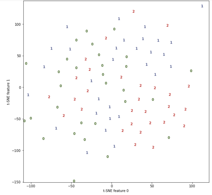
To begin with, we will use the popular T-SNE algorithm (who is curious what it is, you can read it here ).
The main thing for us is that the algorithm displays our data in a two-dimensional plane, and if, in reality, the data are well separable, then in a two-dimensional form they will also be well separable (it will be possible to draw lines and accurately divide the groups).
Unfortunately, everything is not so good here. Somewhere the data is grouped, but somewhere and mixed.
And in principle, this is normal, again, we all know the specifics of the issue , which means that we guess that if the lamps are good, then in their own light they will look like real daylight, and therefore it is difficult to separate the data.
For safety, let's look at the results of the PCA algorithm ( more details here ).
The results are similar.

Well, now let's do direct clustering, there are a lot of algorithms, but for this example we will use the DBSCAN algorithm ( details ).
This algorithm does not require to set the initial number of classes and in some cases allows you to guess well, but running ahead, we remember the pictures from above? In our case it will be difficult. Here is a DBSCAN variant that finds three classes (2 or 4 possible).
Affiliation to clusters:
[-1 -1 0 -1 -1 0 0 -1 1 1 -1 2 2 -1 -1 -1 -1 -1 -1 -1 -1 -1 -1 -1 -1
-1 1 1 1 -1 1 -1 1]
results (clustering, fact):
[(-1, 0), (-1, 0), (0, 0), (-1, 0), (-1, 0), (0, 0), (0, 0), (-1 , 0), (1, 0), (1, 0), (-1, 0), (2, 1), (2, 1), (-1, 1), (-1, 1), ( -1, 1), (-1, 1), (-1, 1), (2, 1), (-1, 1), (2, 1), (-1, 1), (-1, 2), (1, 2), (-1, 2), (-1, 2), (1, 2), (1, 2), (1, 2), (-1, 2), (1 , 2), (-1, 2), (1, 2)]
accuracy_score:
0.0909090909091
We get a terrible accuracy value of about 9%. Something is wrong! Of course, DBSCAN does not know which labels we gave classes, so in our case 1 is 2 and vice versa (a -1 is noise).
Change the class labels and get:
results (clustering, fact):
[(-1, 0), (-1, 0), (0, 0), (-1, 0), (-1, 0), (0, 0), (0, 0), (-1 , 0), (2, 0), (2, 0), (-1, 0), (1, 1), (1, 1), (-1, 1), (-1, 1), ( -1, 1), (-1, 1), (-1, 1), (1, 1), (-1, 1), (1, 1), (-1, 1), (-1, 2), (2, 2), (-1, 2), (-1, 2), (2, 2), (2, 2), (2, 2), (-1, 2), (2 , 2), (-1, 2), (2, 2)]
accuracy_score:
0.393939393939
Another thing is already 39% which is still better than if we were classified in a random way. That's all machine learning, but for patient people at the end of the article there will be a bonus.
Well, we have traveled the hard way from setting the problem to solving it, we confirmed in practice some of the truths that are found in Data Science textbooks.
In fact, we didn’t necessarily have to be categorized by spectral distribution, it was possible to take derived attributes, for example, color rendering index and color temperature, but you can do it yourself if you want.
It also certainly makes sense to add more data to the training and test sample, since the quality of training of the model is very strongly dependent on this (at least in this case, the difference between the sample of 20 and 30 samples was significant).
What do you do with your research when you do it? Well first, you can write an article on Habr :)
And you may not be limited to Habrom, I remember 4 years ago I wrote an article, “How to stop being a“ blogger ”and feel like a“ scientist ” .
Its meaning was that you can not stop at what has been achieved, as a rule, if you are able to write an article on Habr, then you can write to some scientific journal.
What for? Yes, simply because you can! This situation is similar to the game of football, in the RFPL there are about 200 domestic footballers (this is from the ceiling, but I think not much more), and even less of our people play abroad, but in general much more people play football across the country.
After all, there are amateur leagues. Lovers do not get paid, and often play for fun. So here I invite you to play in the "amateur" scientific league.
In our case, if you do not have access to standing international journals, or at least VAK, do not be discouraged, even after the collapse of the RISC, there are places where your good article will be completely accepted, if you observe the formalities and scientific style of presentation, for example, at one of the conferences included in the RSCI , it is usually a pleasure to pay, but very budget.
It will be even more useful to participate in the in-person conference , where you will have to defend your idea live.
Who knows, maybe one day you will put your hand in your mouth and become our new hope for humanity.
There is another use for your talents, you can analyze the data of budget structures and participate in public control, for sure if you dig deeper, there are obvious shoals in the accounts of dishonest people and organizations, and you can make our home better (or not)
Or maybe you will find some more wonderful use of your hobby and wrap it in income, everything is in your hands.
Do not you think that the article remained a little understatement? Something is missing? Well, of course it is necessary to conduct an epic human-machine battle!
Let's see who better classifies the spectra.
Since I do not have this magic cat that guesses everything, I will have to do everything myself.

We write for this a small function. And build graphs for which I will predict.
Note I cannot vouch for the quality of the code
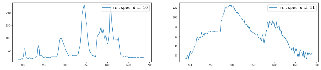
By the way, here is another reference to the man-machine comparison from the 2nd chapter. Frankly, I usually determine the spectra with a photograph of the spectrum and the graph itself at hand, and then the accuracy exceeds 90 and is nearing 100%, but we didn’t give spectra pictures to our model, which means we will have to be on equal terms with it.
This situation is somewhat similar to the one when you are training a model on one set of attributes, and then in real data (or control) some of the signs are missing and the predictive power of the model is greatly reduced (mine has also decreased).
And so take my word for it (or run. Ipynb file with GitHub) we get 33 graphics from the control sample, like these:
Then we manually enter the forecast, return the order order of the labels and see what happens.
Result (my prediction, fact.):
[(0.0, 0), (0.0, 0), (0.0, 0), (1.0, 0), (0.0, 0), (0.0, 0), (0.0, 0), (0.0, 0), ( 0.0, 0), (0.0, 0), (0.0, 0), (1.0, 1), (1.0, 1), (1.0, 1), (1.0, 1), (1.0, 1), (1.0, 1), (1.0, 1), (1.0, 1), (1.0, 1), (1.0, 1), (1.0, 1), (0.0, 2), (2.0, 2), (2.0, 2) , (2.0, 2), (2.0, 2), (2.0, 2), (0.0, 2), (0.0, 2), (2.0, 2), (2.0, 2), (0.0, 2)]
accuracy score = 0.8484848484848485
Of course, I am biased, at least because I know that there are no more than 11 labels in each class in the control sample, but I tried not to cheat.
So, in my first attempt, I got 84% with a little, something between a logistic regression and Random Forest, and the computer went around me in the last position.
Remember at the beginning of the article I mentioned that some of the spectra can be cut off? It was precisely this that let me down, without a photo, I didn’t notice it and incorrectly classified the cut spectrum only according to the schedule, but the computer coped and got its 87%.
If we consider that I have not shone this skill of determining spectra by eye for more than one day, and the model has been trained for a minute or so, then perhaps it’s time to fear the uprising of the machines?

So, for the past several years I have been busy in my spare time in questions related to lighting and most of all I am interested in the spectra of various light sources, like “ancestors” of the characteristics derived from them. But not so long ago, I accidentally had another hobby - machine learning and data analysis, in this matter I am an absolute beginner, and in order to have fun, I periodically share my newfound experience and stuffed "bumps"
This article is written in the style of newbies to beginners , so experienced readers are unlikely to get something new for themselves, and if there is a desire to solve the problem of classifying light sources according to spectra, then it makes sense to immediately get data from GitHub
')
And for those who do not have a great experience, I will suggest continuing our joint training and this time try to take up the task of machine learning, which is called “for yourself”.
We will go with you from trying to understand where you can apply even a little knowledge of ML (which can be obtained from basic books and courses), to solving the very task of classification itself and thinking about "what to do now with all this ?!"
You are welcome all under the cat.
So, colleagues in front of us is a very important mission to find out how dangerous artificial intelligence is, is it time for us to blow up Skynet or can we spend a little more time watching videos with cats.
In this article, we will, on the basis of approximately such images, determine what type of lamp the lamp is in: fluorescent or LED, or perhaps even the light of the sun and sky.
Part 1. Briefing
Let's start with a rather important point , namely with the requirements for skills. As in the previous articles, I share with you the experience that I managed to get myself and before starting the article it is important to understand that it can be useful to people with similar experiences. As I said earlier, material is unlikely to be useful to experienced specialists.
Although they can certainly find some mistakes in it and tell me about it, so that I can correct them if possible.
This time, in order for the article not to cause you difficulties, we already need some basic skills, namely:
- Understanding what Data Science is and why it is needed
- Minimal Python programming skills
If you have taken online courses or have read a self-instruction manual, I think this will be quite enough.
The second important point to understand why we all do it?
Indeed, if you just want to practice analyzing data and solving machine learning problems, then there are many wonderful tasks on Kagle, including those suitable for absolute beginners (for example, about Titanic).
Most likely, these tasks will be more correct and in cases with tasks for beginners you will surely find more successful tutorials than in our case, so if you still do not itch your hands to “invent your own bike” or do not have enough skills, then it makes sense to practice Kagle ( I wrote about this before ).
In the book Data Science from Scratch , closer to the end, the author suggested not dwelling on the materials of the book and coming up with a task on my own, while sharing my ideas, at that moment I thought: “Of course, you are so smart, but I have no idea what to do! ".
In my opinion, this idea was very fair, because it is hard to learn from this book, something very useful in practice ( for more details on this in the review ). And in the end, before sculpting dumplings, it probably makes sense to try them all the same, and it is advisable to try the good ones, so that is what it seeks.
In the Specialization "Machine Learning and Data Analysis", through the eyes of a newbie in Data Science "on Coursera ( review ), there was something to try and get a hand on what, and after passing it, it became certain that now it’s not perfect, but You can collect and analyze data yourself.
Summing up the chapter, I want to say, from a pedagogical point of view, I consider VERY useful and important the stage of self-setting the problem for machine learning, even if it is purely “fake”. That is why I decided to share my example with you.
Part 2. Do not learn to live help financially.
Let's address the question of where to get the material (data) for our research.
In my opinion, the source itself is not so important, the main thing is that the subject matter is close to you and you can find more or less a sufficient amount of reliable data.
Well, for example:
1. You can classify your friends by text messages in the social. networks (someone is silent, someone often uses keywords, someone puts a bunch of emoticons, and so on)
2. Or, based on past data (well, for example, utility bills), you can predict how much hot water or electricity you will spend this November.
3. And you can restore the relationship between the rating of the downloaded series and the number of "snacks" that you eat when viewing it.
4. If you are a very angry person, try to solve the problem of the number of cats in your single friends
5. If you have a hard time with personal experience and you do not store archives in yellowed folders, look at the domestic (or foreign) open data portals data.gov.ru or for Moscow data.mos.ru , for example, you can find the data in order to predict the number of calls of firefighters in a particular district of Moscow in the future, and then check in a couple of months.
In our case, I did not need to go far for data. There is a wonderful opensource project Public Lab, in which there is a subsection devoted to the analysis of the spectrum of light sources .
Two words about him:
The project proposes to assemble a spectroscope from available tools ( well, for example, from cardboard and DVD discs ) and photograph the spectra.
After you take a bunch of spectra images, it would be good to study them in more detail. To do this, they have a web interface on the site that allows you to load and process your spectrum a bit to get a digital view of it (for example, as a table). .
All data is in the public domain, anyone can either download the spectrum to the portal or download data. This openness has one big flaw, which we will need to take into account, but about it a little later (just decided to introduce intrigue into the story) .
There are many pictures on the portal, though it’s important to remember that among the pictures you don’t have to be the spectra of light bulbs, for example, there can be light reflectance spectra of materials or light transmission spectra of various liquids.
In any case, we have visual open data that are unified, structured and most importantly can be downloaded in a convenient format (for example, .csv), what else can you dream of?
(except a million dollars and a personal helicopter)
Part 3. You must think like a car, live like a car, you yourself must become a machine!
Consider the data that we have and what we want to get in the end.
Hereinafter I will focus on the files in the format csv
So we have the distribution of radiation power (conditional) along the wavelength of the spectrum ( spectral distribution of radiation density ).
In the data downloaded from the Public Lab there is an average value as well as broken down by the R, G, B channels, we will only be worried about the average.
If you just simplify the description, then when passing through a diffraction grating or prism, the light splits into a rainbow, and if sunlight gives you a rainbow, as in the saying about the pheasant, then the light of poor-quality fluorescent lamps may look like a hockey player Ovechkin’s smile (certainly charming, but with some spaces) .
It is precisely on the basis of this structure of the rainbow that we will classify the spectra.
Since all algorithms and libraries for machine learning are written by living people (for the time being), in many respects they are a formalization of those things that we often do unconsciously when solving certain tasks.
On the one hand, the data set that I have compiled for you is very simple - the classes are balanced, the signs have a more or less close scale, there are no obvious emissions, so some things that they write in the training materials I cannot demonstrate to you on it.
On the other hand, who knows, maybe we are all robots? Therefore, I will cover a couple of points that would be important to note, as if we had written a model for collecting data instead of doing it manually.
To begin, let us recall the important points that are often talked about and written in educational materials:
Knowledge of the specifics
In the training materials they write that for machine learning it is important to have knowledge of the field of activity for which we are preparing the model. And with this I fully agree, it is not enough to know all the algorithms and methods, to be able to use libraries. Ignorance of some nuances can cover your model with a copper basin and reduce its value to zero.
Let's turn to our case. Remember I talked about the BIG minus of the openness of the platform (with all its advantages). So, people can pour in any photographs of the spectra taken on instruments of any quality, and then process them as they will enter the head.
The most important point to consider is the correct calibration of the spectrum.
The mechanism is as follows: you photograph a characteristic object (a compact fluorescent lamp) and on the basis of it you get a scale of your distribution (based on two peaks of blue and green).
It doesn’t sound very difficult, but you need to tamper a little, firstly, not everyone speaks English, and secondly, not everyone likes to read the instructions, therefore, even now the mechanism has been simplified (by adding a sample), but there is still a risk stumble on an improperly calibrated spectra. In the end, the spectra can be loaded by children and some of them can be hard to figure out on their own.
Therefore, on the one hand, we have a lot of simply uncalibrated images, on the other hand, a certain amount of incorrectly calibrated ones, which is much worse.
For example, there is a photo under it there is a graph like something more or less meaningful (without noise), but naturally this is an incorrect calibration (turquoise should be around 500 nm, and orange around 600 nm.)
This is not the worst example, there are cases where poor calibration is present, but it is much less striking, but I just did not find them without thinking.
The second point is that we don’t really know which spectra (which lamps), under what conditions and what the users photographed them, so at least it’s important to know that you shouldn’t trust the data to 100%. Sometimes some spectra are suspicious.
The third point, it is important to remember about the technical limitations, in most cases, this measuring circuit strongly cuts spectra in the red range of light, therefore, for example, data beyond 600 nm. may not be less reliable and not the fact that they will correspond to the true spectra. The situation is similar with violet (ultraviolet) light.
The fourth point, part of the radiation in the spectra can be cut off, due to the high brightness of the images, this distorts the data and sometimes it can also be important. Maybe there are some other nuances that I did not remember or do not know. So, without knowing even these trifles, it would be possible to make mistakes when preparing the samples.
Signs and data selection
Regarding the signs, let the radiation power for each wavelength be our feature for the future model.
Considering the above, it becomes clear that for classifying us there is not much point in taking the spectrum, in the range that the system gives (sometimes almost from 200 to 1000 nm), take the range from 390 to 690 even this is a bit redundant (because everywhere there is this data), but we don’t seem to lose anything significant.
We divide the signs in steps of 1 nm. Well, for example, 400, 401, 402 ... It would be possible to take a step less often, for example, 10 nm., but we will have a small sample and even 301 signs will not overload our computer when calculating. In theory, increasing the pitch reduces the accuracy of the model, but also drastically reduces the pitch, for example, to 0.25 nm. we do not much weather, and machine resources will eat.
Concerning the selection of spectra
Initially I wanted to make a larger sample with a large number of classes, but it stalled, as I said before, not all spectral images could be used due to poor calibration, noise, or doubts about the reliability.
Therefore, in the end, we limit ourselves to three classes: daylight (sky, sun or all together), fluorescent lamps (both compact and tubular), and LED lamps (white with phosphor and based on RGB LEDs).
I hope that everything that I have gathered to you is shining with white light (of various shades and of different quality).
When collecting data, the problem with poor data calibration for fluorescent lamps was easy to solve; it was enough to calibrate them yourself. But with daylight and LED lamps such a trick will not work (there is often a smooth spectrum), well, at that time I did not find incandescent lamps (calibrated) in sufficient quantities, but new data are actively added there if you consider it necessary to expand the sample and make the task more interesting.
To make it easier to classify as a result, I made the sample uniform. In the training set of 30 records of each class, in the control sample of 11 records.
And even though I was a little tired and confused at the end, the sample should contain examples of different light sources, different lamps, different LEDs, etc.
In this case, I combed the sample for you, but in a real sample, you may have to process the data yourself.
Another point about the sample.
There is such a thing in statistics as errors of the first kind and second kind. In a very simplified presentation: you hypothesize that there is paper in the toilet, which means you don’t take it with you, so if in this situation you insure and take a roll with you in vain (a false positive is a mistake of the first kind), then not as scary as if you don’t grab a roll, and there will only be a cardboard ring (a mistake of the second kind).
So, when choosing data, I tried to minimize the error of the second kind, it was not very scary for us to skip the normal spectrum, but accidentally taking an erroneous spectrum into the sample is clearly not what we need.
But when solving the classification problem directly, any of the errors does not have a higher priority; when it is solved directly by the model, it is important for us that everything is absolutely predicted correctly and without reinsurance.
This is what determines the sufficiency of the metrics accuracy.
Part 4. T-800 and T-1000
Well, there was a lot of text, let's finally move on closer to the model.
At https://github.com/bosonbeard/ML_light_sources_classification/tree/master/1st_spectrum_classification located:
- Train.csv training sample file
- Test sample file test.csv
- Two documents with file names (cut out columns), they will be useful to you if you want to check me and yourself, you can simply take the file name by substituting it to the link, for example, spectralworkbench.org/spectrums/9740 (where 9740 is the file number)
- And the file spectrum_classify_for_habrahabr.ipynb in which is represented in its entirety, the code that we will now consider with you.
I mean that you already have basic knowledge and you will have enough of them to understand my code far from the reference.
Import libraries:
import pandas as pd import numpy as np from sklearn.ensemble import RandomForestClassifier from sklearn.linear_model import LogisticRegression from sklearn.model_selection import GridSearchCV from sklearn.model_selection import StratifiedKFold from sklearn.preprocessing import MinMaxScaler, StandardScaler from sklearn.pipeline import Pipeline from sklearn.decomposition import PCA import matplotlib.pyplot as plt from sklearn.manifold import TSNE from sklearn.cluster import DBSCAN from sklearn.metrics import accuracy_score from IPython.display import display %matplotlib inline Read the data:
#reading data train_df=pd.read_csv('train.csv',index_col=0) test_df=pd.read_csv('test.csv',index_col=0) print('train shape {0}, test shape {1}]'. format(train_df.shape, test_df.shape)) #divide the data and labels X_train=np.array(train_df.iloc[:,:-1]) X_test=np.array(test_df.iloc[:,:-1]) y_train=np.array(train_df['label']) y_test=np.array(test_df['label']) In this case, we use the pandas library and its dataframe class, which, to put it simply, gives us the functions that Excel would give, that is, work with tables.
As I said earlier, in table 391 the column corresponds to the radiation power by wavelength, and the last column is the class label: 0 - LED, 1 - lum. lamps. 2 - daylight.
For further work, we immediately cut out 391 columns with signs and the last columns with labels into separate variables.
In normal work, a decent analysis of the initial data usually goes on, but we have nothing to analyze, as I said, all classes are balanced and, in principle, do not need much additional scaling (although you can scale it out of curiosity).
#draw classdistributions fig, axes = plt.subplots(nrows=1, ncols=2, figsize=(12,5)) train_df.label.plot.hist(ax=axes[0],title='train data class distribution', bins=5,xticks=np.unique(train_df.label.values)) test_df.label.plot.hist(ax=axes[1],title='test data class distribution',bins=5,xticks=np.unique(test_df.label.values)) For the sake of form, I derived 2 graphics, if you want you can do something else.
Classification
Let's build our first model. Take one of the most popular models - the random forest model (decisive trees).
rfc = RandomForestClassifier(n_estimators=30, max_depth=5, random_state=42, n_jobs=-1) rfc.fit(X_train, y_train) pred_rfc=rfc.predict(X_test) print("results (predict, real): \n",list(zip(pred_rfc,y_test))) print("accuracy score= {0}".format(rfc.score(X_test,y_test))) Let's see the results.
(predicted, actual):
(2, 0), (0, 0), (0, 0), (0, 0), (0, 0), (0, 0), (1, 0), (0, 0), (2 , 0), (2, 0), (2, 0), (1, 1), (1, 1), (1, 1), (1, 1), (0, 1), (1, 1 ), (1, 1), (1, 1), (1, 1), (1, 1), (1, 1), (2, 2), (2, 2), (2, 2), (2, 2), (2, 2), (2, 2), (2, 2), (2, 2), (2, 2), (2, 2), (2, 2)
Accuracy prediction (share of correct answers) = 0.8181818181818182
It turns out we can hope that our model will be 8 out of 10 spectra correctly classified, which is already good.
For the demonstration, we specifically took the best parameters for this model, let's try to sort through models with different parameters and select the best one based on the results of cross-checking.
%%time param_grid = {'n_estimators':[10, 20, 30, 40, 50], 'max_depth':[4,5,6,7,8]} grid_search_rfc = GridSearchCV(RandomForestClassifier(random_state=42,n_jobs=-1), param_grid, cv=7) grid_search_rfc.fit(X_train, y_train) print(grid_search_rfc.best_params_,grid_search_rfc.best_score_) print("best accuracy on cv: {:.2f}".format(grid_search_rfc.best_score_)) print("accuracy on test data: {:.5f}".format(grid_search_rfc.score(X_test, y_test))) print("best params: {}".format(grid_search_rfc.best_params_)) print("results (predict, real): \n",list(zip(grid_search_rfc.best_estimator_.predict(X_test),y_test))) We get the following parameters:
{'max_depth': 6, 'n_estimators': 30} 0.766666666667
best accuracy on cv: 0.77
accuracy on test data: 0.87879
best params: {'max_depth': 6, 'n_estimators': 30}
(predicted, actual):
[(0, 0), (0, 0), (0, 0), (0, 0), (0, 0), (0, 0), (0, 0), (0, 0), ( 2, 0), (2, 0), (2, 0), (1, 1), (1, 1), (1, 1), (1, 1), (0, 1), (1, 1), (1, 1), (1, 1), (1, 1), (1, 1), (1, 1), (2, 2), (2, 2), (2, 2) , (2, 2), (2, 2), (2, 2), (2, 2), (2, 2), (2, 2), (2, 2), (2, 2)]
Wall time: 1min 6s
That is, an increase of max_depth by 1 improves accuracy by 6%, which is not bad, despite the fact that the model with the number of trees (n_estimators), like “you will not spoil the porridge with oil,” the model decided that it is not worth further increasing their number (this saves resources).
I think you can achieve better results if you search for more parameters (or increase the sample size), but in order to demonstrate that the calculation does not take much time, we will limit ourselves to what it is.
So, you and I can start with our more advanced T-1000, so let's try to force something to classify our “Iron Arnie” as a simpler Logistic Regression model.
logreg = LogisticRegression(penalty='l2',random_state=42, C=1, n_jobs=-1) logreg.fit(X_train, y_train) pred_logreg = logreg.predict(X_test) print("results (predict, real): \n",list(zip(pred_logreg,y_test))) print("accuracy score= {0}".format(logreg.score(X_test,y_test))) As one would expect, the simpler model from the first approach gave a little worse result.
results (predict, real):
[(0, 0), (0, 0), (0, 0), (2, 0), (0, 0), (0, 0), (0, 0), (2, 0), ( 0, 0), (0, 0), (2, 0), (1, 1), (1, 1), (1, 1), (1, 1), (2, 1), (2, 1), (1, 1), (1, 1), (1, 1), (1, 1), (2, 1), (2, 2), (2, 2), (2, 2) , (0, 2), (2, 2), (2, 2), (2, 2), (2, 2), (2, 2), (2, 2), (2, 2)]
accuracy score = 0.7878787878787878
We can play again with the parameters:
%%time param_grid = {'C':[0.00020, 0.0020, 0.020, 0.20, 1.2], 'penalty':['l1','l2']} grid_search_logr = GridSearchCV(LogisticRegression(random_state=42,n_jobs=-1), param_grid, cv=3) grid_search_logr.fit(X_train, y_train) print("best accuracy on cv: {:.2f}".format(grid_search_logr.best_score_)) print("accuracy on test data: {:.5f}".format(grid_search_logr.score(X_test, y_test))) print("best params: {}".format(grid_search_logr.best_params_)) print("results (predict, real): \n",list(zip(grid_search_logr.best_estimator_.predict(X_test),y_test))) Results:
best accuracy on cv: 0.79
accuracy on test data: 0.81818
best params: {'C': 0.02, 'penalty': 'l1'}
(predicted, actual):
[(0, 0), (0, 0), (0, 0), (2, 0), (0, 0), (0, 0), (0, 0), (0, 0), ( 0, 0), (0, 0), (2, 0), (1, 1), (1, 1), (1, 1), (1, 1), (2, 1), (2, 1), (1, 1), (1, 1), (1, 1), (1, 1), (2, 1), (2, 2), (2, 2), (2, 2) , (0, 2), (2, 2), (2, 2), (2, 2), (2, 2), (2, 2), (2, 2), (2, 2)]
Wall time: 718 ms
So, we have achieved a quality comparable to Random forest without fitting the parameters, but we have spent significantly less time. It is seen precisely for this reason in the books they write that logistic regression is often used at the preliminary stages, when it is important to identify general patterns, and 5-7% of the weather will not be done right away.
On the one hand, this could be the end, but let's also try to imagine that I, as a dishonest person, gave you data without any description and you need to try to understand something without having class marks.
Clustering
For clarity, let's set the colors. I'm still a little cunning, in an amicable way, “we don’t know” that we have no more than three classes, but we really do know that, so we’ll confine ourselves to three colors.
colors = ["#476A2A", "#535D8E", "#BD3430"] To begin with, we will try to look at our data, we have almost 400 signs and on the two-dimensional sheet of paper all of them probably will not be able to be displayed even by great magicians and wizards Amayak Hakobyan and Harry Potter, but thank God we have the magic of special libraries.
To begin with, we will use the popular T-SNE algorithm (who is curious what it is, you can read it here ).
The main thing for us is that the algorithm displays our data in a two-dimensional plane, and if, in reality, the data are well separable, then in a two-dimensional form they will also be well separable (it will be possible to draw lines and accurately divide the groups).
Unfortunately, everything is not so good here. Somewhere the data is grouped, but somewhere and mixed.
And in principle, this is normal, again, we all know the specifics of the issue , which means that we guess that if the lamps are good, then in their own light they will look like real daylight, and therefore it is difficult to separate the data.
#T-SNE tsne = TSNE(random_state=42) d_tsne = tsne.fit_transform(X_train) plt.figure(figsize=(10, 10)) plt.xlim(d_tsne[:, 0].min(), d_tsne[:, 0].max() + 10) plt.ylim(d_tsne[:, 1].min(), d_tsne[:, 1].max() + 10) for i in range(len(X_train)): # , plt.text(d_tsne[i, 0], d_tsne[i, 1], str(y_train[i]), color = colors[y_train[i]], fontdict={'weight': 'bold', 'size': 10}) plt.xlabel("t-SNE feature 0") plt.ylabel("t-SNE feature 1") For safety, let's look at the results of the PCA algorithm ( more details here ).
#PCA pca = PCA(n_components=2, random_state=42) pca.fit_transform(X_train) d_pca = pca.transform(X_train) plt.figure(figsize=(10, 10)) plt.xlim(d_pca[:, 0].min(), d_pca[:, 0].max() + 130) plt.ylim(d_pca[:, 1].min(), d_pca[:, 1].max() + 30) for i in range(len(X_train)): # , plt.text(d_pca[i, 0], d_pca[i, 1], str(y_train[i]), color = colors[y_train[i]], fontdict={'weight': 'bold', 'size': 10}) plt.xlabel("1-st main comp.") plt.ylabel("2-nd main comp.") The results are similar.
Well, now let's do direct clustering, there are a lot of algorithms, but for this example we will use the DBSCAN algorithm ( details ).
This algorithm does not require to set the initial number of classes and in some cases allows you to guess well, but running ahead, we remember the pictures from above? In our case it will be difficult. Here is a DBSCAN variant that finds three classes (2 or 4 possible).
#scale data scaler = MinMaxScaler() scaler.fit(X_test) X_scaled = scaler.transform(X_test) #clustering with DBSCAN dbscan = DBSCAN(min_samples=2, eps=2.22, n_jobs=-1) clusters = dbscan.fit_predict(X_scaled) print("Affiliation to clusters:\n{}".format(clusters)) print("\n results (Clustering, real): \n",list(zip(clusters,y_test))) print("\n accuracy_score: \n",accuracy_score(clusters,y_test)) Affiliation to clusters:
[-1 -1 0 -1 -1 0 0 -1 1 1 -1 2 2 -1 -1 -1 -1 -1 -1 -1 -1 -1 -1 -1 -1
-1 1 1 1 -1 1 -1 1]
results (clustering, fact):
[(-1, 0), (-1, 0), (0, 0), (-1, 0), (-1, 0), (0, 0), (0, 0), (-1 , 0), (1, 0), (1, 0), (-1, 0), (2, 1), (2, 1), (-1, 1), (-1, 1), ( -1, 1), (-1, 1), (-1, 1), (2, 1), (-1, 1), (2, 1), (-1, 1), (-1, 2), (1, 2), (-1, 2), (-1, 2), (1, 2), (1, 2), (1, 2), (-1, 2), (1 , 2), (-1, 2), (1, 2)]
accuracy_score:
0.0909090909091
We get a terrible accuracy value of about 9%. Something is wrong! Of course, DBSCAN does not know which labels we gave classes, so in our case 1 is 2 and vice versa (a -1 is noise).
Change the class labels and get:
def swap_class(lst, number_one,number_two ): """ The function is exchanging num1 and num2 in list and return new array """ lst_new=[] for val in lst: if val == number_one: val = number_two elif val == number_two: val = number_one lst_new.append(val ) return np.array(lst_new) y_changed=swap_class(clusters, 1,2) print("\n results (Clustering, real): \n",list(zip(y_changed,y_test))) print("\n accuracy_score: \n",accuracy_score(y_changed,y_test)) results (clustering, fact):
[(-1, 0), (-1, 0), (0, 0), (-1, 0), (-1, 0), (0, 0), (0, 0), (-1 , 0), (2, 0), (2, 0), (-1, 0), (1, 1), (1, 1), (-1, 1), (-1, 1), ( -1, 1), (-1, 1), (-1, 1), (1, 1), (-1, 1), (1, 1), (-1, 1), (-1, 2), (2, 2), (-1, 2), (-1, 2), (2, 2), (2, 2), (2, 2), (-1, 2), (2 , 2), (-1, 2), (2, 2)]
accuracy_score:
0.393939393939
Another thing is already 39% which is still better than if we were classified in a random way. That's all machine learning, but for patient people at the end of the article there will be a bonus.
Part 5. Conclusion
Well, we have traveled the hard way from setting the problem to solving it, we confirmed in practice some of the truths that are found in Data Science textbooks.
In fact, we didn’t necessarily have to be categorized by spectral distribution, it was possible to take derived attributes, for example, color rendering index and color temperature, but you can do it yourself if you want.
It also certainly makes sense to add more data to the training and test sample, since the quality of training of the model is very strongly dependent on this (at least in this case, the difference between the sample of 20 and 30 samples was significant).
What do you do with your research when you do it? Well first, you can write an article on Habr :)
And you may not be limited to Habrom, I remember 4 years ago I wrote an article, “How to stop being a“ blogger ”and feel like a“ scientist ” .
Its meaning was that you can not stop at what has been achieved, as a rule, if you are able to write an article on Habr, then you can write to some scientific journal.
What for? Yes, simply because you can! This situation is similar to the game of football, in the RFPL there are about 200 domestic footballers (this is from the ceiling, but I think not much more), and even less of our people play abroad, but in general much more people play football across the country.
After all, there are amateur leagues. Lovers do not get paid, and often play for fun. So here I invite you to play in the "amateur" scientific league.
In our case, if you do not have access to standing international journals, or at least VAK, do not be discouraged, even after the collapse of the RISC, there are places where your good article will be completely accepted, if you observe the formalities and scientific style of presentation, for example, at one of the conferences included in the RSCI , it is usually a pleasure to pay, but very budget.
It will be even more useful to participate in the in-person conference , where you will have to defend your idea live.
Who knows, maybe one day you will put your hand in your mouth and become our new hope for humanity.
There is another use for your talents, you can analyze the data of budget structures and participate in public control, for sure if you dig deeper, there are obvious shoals in the accounts of dishonest people and organizations, and you can make our home better (or not)
Or maybe you will find some more wonderful use of your hobby and wrap it in income, everything is in your hands.
Bonus Manual forecast
Do not you think that the article remained a little understatement? Something is missing? Well, of course it is necessary to conduct an epic human-machine battle!
Let's see who better classifies the spectra.
Since I do not have this magic cat that guesses everything, I will have to do everything myself.
We write for this a small function. And build graphs for which I will predict.
Note I cannot vouch for the quality of the code
def print_spec_rand(data): """ the function takes a DataFrame and returns in random order the x-coordinate (wavelength), the power values for all light sources (the y-axis), and the matching to the original DataFrame positions. Use it for manual prediction. """ x=data.columns.values[:-1] data_y=data.values y=list() pos=list() rows_count=data_y.shape[0] index=range(0,rows_count+1) while rows_count>1: rows_count=data_y.shape[0] i=np.random.randint(0,data_y.shape[0]) y.append(data_y[i][:-1]) pos.append(index[i]) data_y=np.delete(data_y, i, 0) index=np.delete(index, i, 0) #print (len(data_y,)) return x, y, pos def get_match_labels(human_labels, pos_in_data_lebels): """ The function returns a match between the random data and the original DataFrame """ match=np.zeros(len(human_labels)) for h,p in zip (human_labels, pos_in_data_lebels): match[p]=h return match By the way, here is another reference to the man-machine comparison from the 2nd chapter. Frankly, I usually determine the spectra with a photograph of the spectrum and the graph itself at hand, and then the accuracy exceeds 90 and is nearing 100%, but we didn’t give spectra pictures to our model, which means we will have to be on equal terms with it.
This situation is somewhat similar to the one when you are training a model on one set of attributes, and then in real data (or control) some of the signs are missing and the predictive power of the model is greatly reduced (mine has also decreased).
And so take my word for it (or run. Ipynb file with GitHub) we get 33 graphics from the control sample, like these:
Then we manually enter the forecast, return the order order of the labels and see what happens.
# my prediction, as an example man_ped=[0,1,2,0,1,1,2,0,0,1,0,1,1,2,0,0,2,1,1,0,1,1,0,0,0,0,1,2,1,0,2,0,2] man_pred_trans=get_match_labels(man_ped, pos) print("results (predict, real): \n",list(zip(man_pred_trans,y_test))) print("accuracy score= {0}".format(accuracy_score(man_pred_trans,y_test))) Result (my prediction, fact.):
[(0.0, 0), (0.0, 0), (0.0, 0), (1.0, 0), (0.0, 0), (0.0, 0), (0.0, 0), (0.0, 0), ( 0.0, 0), (0.0, 0), (0.0, 0), (1.0, 1), (1.0, 1), (1.0, 1), (1.0, 1), (1.0, 1), (1.0, 1), (1.0, 1), (1.0, 1), (1.0, 1), (1.0, 1), (1.0, 1), (0.0, 2), (2.0, 2), (2.0, 2) , (2.0, 2), (2.0, 2), (2.0, 2), (0.0, 2), (0.0, 2), (2.0, 2), (2.0, 2), (0.0, 2)]
accuracy score = 0.8484848484848485
Of course, I am biased, at least because I know that there are no more than 11 labels in each class in the control sample, but I tried not to cheat.
So, in my first attempt, I got 84% with a little, something between a logistic regression and Random Forest, and the computer went around me in the last position.
Remember at the beginning of the article I mentioned that some of the spectra can be cut off? It was precisely this that let me down, without a photo, I didn’t notice it and incorrectly classified the cut spectrum only according to the schedule, but the computer coped and got its 87%.
If we consider that I have not shone this skill of determining spectra by eye for more than one day, and the model has been trained for a minute or so, then perhaps it’s time to fear the uprising of the machines?
Source: https://habr.com/ru/post/337040/
All Articles