History of predictions of transitions from 1 500 000 BC. till 1995
This is an approximate transcript of a lecture on predicting transitions (branch prediction) to localhost, a new lecture series organized by RC . The performance took place on August 22, 2017 at Two Sigma Ventures.
Who among you uses branching in your code? Can you raise your hand if you use if statements or pattern matching?
Now I will not ask you to raise your hands. But if I ask how many of you think that you understand the actions of the CPU when processing branching and the implications for performance, and how many of you can understand a modern scientific article on branch prediction, fewer people will raise their hands.
')
The purpose of my presentation is to explain how and why processors predict transitions, and then briefly explain the classic transition prediction algorithms that you can read about in modern articles so that you have a general understanding of the topic.
Before discussing the prediction of transitions, let's talk about why processors do this at all. To do this, you need to know a little about the work of the CPU.
In this lecture you can think of a computer as a CPU plus some memory. Instructions live in memory, and the CPU executes a sequence of instructions from memory, where the instructions themselves look like “add two numbers”, “transfer a piece of data from memory to the processor”. Usually, after executing one instruction, the CPU executes the instruction with the next address in order. However, there are instructions such as "transitions" that allow you to change the address of the next instruction.
Here is an abstract diagram of a CPU that executes some instructions. Time is plotted on the horizontal axis, and differences between different instructions are on the vertical axis.
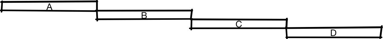
Here we first execute instruction A, then instruction B, C and D.
One way to design a CPU is to do all the work in turn. There is nothing wrong with that; Many old CPUs work like some modern, very cheap processors. But if you want to make a faster CPU, then you need to turn it into a kind of pipeline. To do this, you break the processor into two parts, so that the first half is on the frontend of working with instructions, and the second half is in the backend, like on a conveyor belt. This is commonly referred to as a pipelined CPU (pipelined processor).
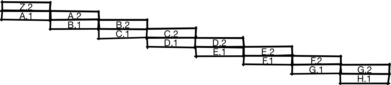
If you do this, then the instructions will be executed approximately as in the illustration. After the first half of instruction A is executed, the processor starts working on the second half of instruction A simultaneously with the first half of instruction B. And when the second half of A is completed, the processor can simultaneously start the second half of B and the first half of C. In this diagram, you can see that the pipeline processor able to perform in a period of time twice as many instructions as a conventional processor, as shown earlier.
There is no reason to split the CPU into just two parts. We can divide it into three parts and get a threefold increase in productivity or four parts for a fourfold increase. Although this is not quite true and in fact usually the increase will not be threefold for a three-stage conveyor or fourfold for a four-stage conveyor, because there are certain overhead costs when dividing the CPU into parts.
One source of overhead is how branches are processed. First of all, the CPU should receive instructions. For this, he must know where she is. For example, take the following code:
It can be translated into assembler:
In this example, we compare x with zero. If it is not equal to zero (
For the pipeline, the specific sequence of instructions is problematic:
The processor does not know what will happen next:
or
He does not know this until the execution of the branch has been completed (or almost completed). One of the first actions of the CPU should be to retrieve the instruction from the memory, and we do not even know what the instruction will be
Earlier we said that we get almost threefold acceleration when using a three-stage conveyor, or almost 20-fold when using a 20-step. It was assumed that on each cycle you can begin executing the new instruction, but in this case the two instructions are practically serialized.
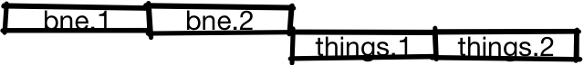
One solution to the problem is to use the prediction of transitions. When a branch appears, the CPU will assume whether this branch is taken or not.
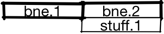
In this case, the processor predicts that the branch will not be busy, and begins the execution of the first half of the

If the prediction is erroneous, then after completion of the execution of the branch, the CPU will discard the results of
What is the performance impact? To evaluate it, you need to simulate performance and load. For this lecture, we take a caricature model of a conveyor CPU, where non-branching is worked out in approximately one instruction per cycle, unpredicted or incorrectly predicted transitions take 20 cycles, and correctly predicted transitions take one cycle.
If we take the most popular benchmark for integer loads on the SPECint "workstation", then the distribution can be 20% of branches and 80% of other operations. Without a prediction of transitions, we expect that the “average” instruction will take
See what you can do about it. Let's start with the simplest things, and gradually develop a better solution.
Instead of random predictions, we can look at all the branches of the execution of all programs. In this case, we will see that taken and unmarked branches are not equally balanced - the branches taken are much more than the uncivilized ones. One of the reasons are loop branches that are often executed.
If we predict the taking of each branch, then we can reach the level of prediction accuracy of 70%, so we will only pay for incorrectly predicted 30% of transitions, which reduces the cost of the average instruction to

Predicting the taking of all branches works well for cycles, but not for other branches. If you look at the percentage of transitions carried forward in the program or back in the program (returning to the previous code), we will see that the transitions are performed more often than the transitions forward. Therefore, you can try a predictor that predicts taking all transitions back and not taking all transitions forward (BTFNT, backwards taken forwards not taken). If we implement this scheme at the hardware level, the compilers will adapt to us and begin to organize the code so that the branches with the greatest chances of execution become transitions back, and the branches with the least chances of execution become transitions forward.
If you do this, you can achieve prediction accuracy of about 80%, which reduces the cost of executing instructions to

Who uses:
So far, we have considered schemes that do not save any state, that is, such schemes, where the predictor ignores the program execution history. In the literature, they are called static transition prediction methods. Their advantage is simplicity, but they do poorly with predicting transitions that change over time. Here is an example of such a transition:
During the execution of the program at one stage, the flag can be set and the transition is made, and at another stage there is no flag and the transition does not occur. Static methods cannot predict branching like this well, so consider dynamic methods, where the prediction may vary depending on the execution history of the program.
One of the simplest things is to predict on the basis of the last result, that is, to predict the transition if it took place the last time, and vice versa.
Since assigning a bit to each transition is too much for reasonable storage, we will make a table for a certain number of transitions that have taken place recently. For this lecture, assume that the absence of a transition corresponds to 0, and the capture of a branch is 1.
In our case, so that everything fits in the illustration, take a table with 64 entries. This number of records allows us to index the table with 6 bits, so that we use the lower 6 bits of the jump address. After the transition is completed, we update the state in the prediction table (highlighted below), and the next time in the index we use the already updated state.
Perhaps there will be an overlap and two branches from different places will point to the same address. The scheme is not perfect, but it is a compromise between the speed of the table and its size.
If you use a one-bit scheme, then we can achieve an accuracy of 85%, which corresponds to an average

Who uses:
A one-bit scheme works well for templates of the form
The “saturating” part of the counter means that if we count to 00, then we remain at this value. In the same way, if we count to 11, then we stay on it. This scheme is identical to one bit, but instead of one bit in the prediction table, we use two bits.
Compared to a single-bit scheme, a two-bit scheme can have half the number of records at the same size and cost (if we take into account only the cost of storage, but do not take into account the cost of the counter logic). But even so, for any reasonable table size, a two-bit scheme provides better accuracy.
Despite its simplicity, the scheme works quite successfully, and we can expect an increase in accuracy in the two-bit predictor to about 90%, which corresponds to 1.38 cycles per instruction.

It seems logical to generalize the scheme for an n-bit counter with saturation, but it turns out that increasing the bit depth has almost no effect on accuracy. We did not discuss the price of the branch predictor, but the transition from two to three bits increases the size of the table by a factor of one and a half for insignificant gain. In most cases it is not worth it. The simplest and most common cases that we cannot predict well with a two-bit predictor are patterns like
Who uses:
If you think about this code
Then it generates a branch pattern like
If we know the three previous branch results, then we can predict the fourth:
The previous schemes used the branch address to place the index in a table that indicated whether or not a transition was more likely depending on the program execution history. She says in which direction the branching will take place, but she is not able to guess that we are in the middle of a repeating pattern. To fix this, we will keep the history of most recent transitions, as well as a table of predictions.
In this example, we associate the four bits of the transition history with two bits of the transition address to place the index in the prediction table. As before, the source of the prediction is a two-bit counter with saturation. Here we do not want to use only the conversion history for the index. If you do this, then any two branches with the same history will refer to the same entry in the table. In a real predictor, we would probably have a larger table and more bits for the jump address, but we have to use a six-bit index to fit the table into the slide.
Below we see what value is updated during the transition.
Bold highlighted upgradeable parts. In this diagram, we shift the new bits of the transition history from right to left, updating the branch history. As the history is updated, the lower bits of the index in the prediction table are also updated, so the next time we encounter this branch, we use a different value from the table to predict the transition, unlike previous schemes, where the index was fixed in the transition address.
Since the global history is stored in this diagram, it will correctly predict patterns like
If there is a transition along the first or second branch, the third one will definitely remain untapped.
With this scheme, we can achieve an accuracy of 93%, which corresponds to 1.27 cycles per instruction.

Who uses:
As mentioned above, the global history scheme has the problem that the history of local branches is clogged by other branches.
Good local predictions can be achieved by storing the history of local branches separately.

Instead of storing a single global history, we save a table of local histories, indexed by the address of the transition. Such a scheme is identical to the global scheme that we have just considered, with the exception of storing the histories of several branches. You can imagine a global history as a special case of a local history, where the number of stored stories is 1.
With this scheme, we can achieve an accuracy of 94%, which corresponds to 1.23 cycles per instruction

Who uses:
In the global two-tier scheme, you have to compromise: in the fixed-size prediction table, the bits must match either the transition history or the transition address. We would like to allocate more bits for the transition history, because this will allow us to track the correlations at a greater distance, as well as to track more complex patterns. But we also want to give more bits under the address to avoid mutual interference between unrelated branches.
You can try to solve both problems by applying simultaneous hashing, and not the linkage of the transition history and the address of the transition. This is one of the simplest and most reasonable things we can do, and the first candidate for the role of the mechanism for this operation comes
With this scheme, we can increase the accuracy to about 94%. This is the same accuracy as in the local scheme, but gshare does not need to store a large table of local stories.That is, we get the same accuracy at lower cost, which is a significant improvement.
Who uses:
One of the reasons for incorrect prediction of transitions is interference between different branches that refer to the same address. There are many ways to reduce interference. In fact, in this lecture we look at the schemes of the 90s precisely because since then a large number of noise suppression schemes have been proposed, and there are too many of them to meet the half hour.
Let's look at one scheme that gives a general idea of how interference elimination may look like - this is the “agree” predictor. When a collision of two history-transition pairs occurs, the predictions either coincide or not. If they match, we call it neutral interference, and if not, then negative interference. The idea is that most of the branches have a strong bias in some way (that is, if we use a two-bit entry in the table of predictions, it is expected that most of the entries without interference most of the time will be equal to
If you look at how this works, then the predictor is identical to the gshare predictor, with the exception of the change we made - the prediction now looks like agree / disagree (agree or disagree), not taken / not taken (transition made or not implemented) , and we have the “bias” bit, which is indexed at the jump address, which gives us the material to make an agree / disagree decision. The authors of the original scientific article suggest using “bias” directly, but other experts have put forward the idea of defining “bias” by optimization based on profiling (essentially, when a working program sends data back to the compiler).
Notice that if we make the transition and then go back to the same branch, we will use the same bit “bias” because it is indexed by the transition address, but we will use another entry in the prediction table because it is indexed at the same time and the address of the transition, and the history of transitions.

If it seems strange to you that such a change matters, consider it with a specific example. Let's say we have two branches, branch A, on which the transition occurs with a probability of 90%, and branch B, on which the transition occurs with a probability of 10%. If we assume that the probabilities of transitions for each branch are independent of each other, then the probability of a disagree decision and negative interference is
If we use the agree scheme, we can repeat this calculation, but the probability of a disagree decision making for the two branches and negative interference is
With this scheme, we can achieve an accuracy of 95%, which corresponds to 1.19 cycles per instruction.

Who uses:
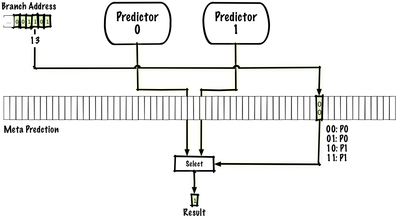
As we have seen, local predictors can well predict some types of branching (for example, built-in loops), and global predictors do well with other types (for example, with some correlated branches). You can try to combine the advantages of both predictors and get a meta-predictor that predicts whether to use a local or global predictor. A simple way is to use the same scheme for a meta-predictor as in the above-described two-bit predictor, but instead of a prediction,
Also, as there are many schemes for eliminating interference, one of which is the aforementioned agree scheme, there are also many hybrid schemes. We can use any two predictors, not only local and global, and the number of predictors is even more than two.
If we use global and local predictors, we can achieve an accuracy of 96%, which corresponds to a 1.15 cycle per instruction.

Who uses:
In this lecture, we have not talked about many things. As you might expect, the volume of the leaked material is much larger than the one we told you about. I will briefly mention some of the missing topics with links, so you can read about them if you want to know more.
One important thing we didn’t talk about was how to predict the destination of the transition . Note that this needs to be done even for some unconditional transitions (that is, for transitions that do not need special prediction, because they occur in any case), because (some) unconditional transitions have unknown goals .
Predicting the goal of a transition is so costly that some early CPUs had a transition prediction policy “to always predict no transition”, because the target address of the transition is not needed if there is no transition! Constant prediction of the absence of transitions has low accuracy, but it is still higher than if you do not make predictions at all.
Among the predictors with reduced interference, which we have not discussed, bi-mode , gskew and YAGS. Briefly, bi-mode is similar to agree in trying to split transitions by direction, but it uses a different mechanism: we maintain several prediction tables, and the third predictor uses the transition address to predict which table to use for a particular transition combination. and transition history. Bi-mode seems to be more successful than agree, as it has gained wider use. In the case of gksew, we maintain at least three prediction tables and separate hashes for indexing each table. The idea is that if two transitions overlap each other in the index, then this only happens in one table, so that we can vote and the result from the other two tables overlap the potentially bad result from the overlapping table. I do not know how to very briefly describe the scheme YAGS :-).
Since we did not talk about speed (delay), we did not talk about such a prediction strategy as using a small / fast predictor, the result of which can be covered by a slower and more accurate predictor.
Some modern CPUs have completely different conversion predictors; AMD Zen (2017) and AMD Bulldozer (2011) processors seem to use perceptron transition predictors . Perceptrons are single-level neural networks.
Allegedly , the Intel Haswell processor (2013) uses a variation of the TAGE predictor. TAGE means tagged geometric (TAgged Geometric) predictor with history size. If we study the predictors described by us and look at the actual execution of programs — which transitions are predicted incorrectly there, then there is one big class among them: these are transitions that need a big story. A significant number of transitions require dozens or hundreds of bits of history, and some even need more than a thousand bits of conversion history. If we have a single predictor or even a hybrid one that combines several different predictors, it will be inefficient to store a thousand bits of history, since this reduces the quality of predictions for transitions that need a relatively small history (especially in relation to price), and most of such transitions. One of the ideas behind the TAGE predictor is thatto keep the geometric lengths of the story sizes, and then each transition will use the corresponding story. This is an explanation of a part of GE in the abbreviation. The TA part means that the transitions are tagged. We did not discuss this mechanism; the predictor uses it to determine which story corresponds to which transitions.
In modern CPUs, specialized predictors are often used. For example, the cycle predictor can accurately predict transitions in cycles where the general transition predictor is not able to store a reasonable history size for perfect prediction of each iteration of the cycle.
We didn’t talk at all about the trade-off between memory usage and better predictions. Changing the size of the table not only changes the effectiveness of the predictor, but also changes the balance of forces in which predictor is better compared to others.
We also did not talk at all about how different tasks affect the performance of predictors of different types. Their effectiveness depends not only on the size of the table, but also on which particular program is running.
We also discussed the cost of incorrectly predicting a transition as if it were a constant value, but this was not the case , and in this respect the cost of instructions without transitions is also very different, depending on the type of task being performed.
I tried to avoid confusing terminology where possible, so if you read the literature, there is a slightly different terminology.
We reviewed a number of classical predictors of transitions and very briefly discussed a couple of newer predictors. Some of the classic predictors we considered are still used in processors, and if I had an hour of time, not half an hour, we could discuss the most up-to-date predictors. I think many people have the idea that a processor is a mysterious and difficult to understand thing, but in my opinion, processors are actually easier to understand than software. I may not be objective, because I used to work with processors, but still it seems to me that this is not my bias, but this is something fundamental.
If you think about the complexity of the software, then the only limiting factor of this complexity will be your imagination. If you can imagine something in such detailed detail that it can be recorded, then you can do it. Of course, in some cases the limiting factor is something more practical (for example, the performance of large-scale applications), but I think most of us spend most of the time writing programs, where the limiting factor is the ability to create and manage complexity.
The hardware is noticeably different here, because there are forces that oppose complexity. Every piece of iron you implement costs money, so you want to use a minimum of equipment. In addition, for most iron, performance is important (whether it is absolute performance or productivity per dollar, or per watt, or other resource), and the increase in complexity slows down the iron, which limits productivity. Today you can buy a serial CPU for $ 300, which accelerates to 5 GHz. At 5 GHz, one unit of work is performed in one fifth of a nanosecond. For information, light travels about 30 centimeters per nanosecond. Another deterrent is that people get very upset if the CPU doesn't work perfectly all the time. Although processors have bugs, the number of bugs is much less than in almost any software, that is, the standards for checking / testing them are much higher. Increasing complexity makes testing and verification difficult. Since processors adhere to a higher standard of accuracy than most software , increasing the complexity adds too much testing / testing burden for the CPU. Thus, the same complication is much more expensive for hardware than for software, even without taking into account other factors that we discussed.
A side effect of these factors that counteract the complexity of the chip is that each “high-level” function of a general-purpose processor is usually fairly conceptually simple to describe in half an hour or an hour lecture. Processors are simpler than many programmers think! By the way, I said “high-level” to exclude all sorts of things like devices of transistors and circuitry, for understanding of which a certain low-level background is needed (physics or electronics).
Who among you uses branching in your code? Can you raise your hand if you use if statements or pattern matching?
Now I will not ask you to raise your hands. But if I ask how many of you think that you understand the actions of the CPU when processing branching and the implications for performance, and how many of you can understand a modern scientific article on branch prediction, fewer people will raise their hands.
')
The purpose of my presentation is to explain how and why processors predict transitions, and then briefly explain the classic transition prediction algorithms that you can read about in modern articles so that you have a general understanding of the topic.
Before discussing the prediction of transitions, let's talk about why processors do this at all. To do this, you need to know a little about the work of the CPU.
In this lecture you can think of a computer as a CPU plus some memory. Instructions live in memory, and the CPU executes a sequence of instructions from memory, where the instructions themselves look like “add two numbers”, “transfer a piece of data from memory to the processor”. Usually, after executing one instruction, the CPU executes the instruction with the next address in order. However, there are instructions such as "transitions" that allow you to change the address of the next instruction.
Here is an abstract diagram of a CPU that executes some instructions. Time is plotted on the horizontal axis, and differences between different instructions are on the vertical axis.
Here we first execute instruction A, then instruction B, C and D.
One way to design a CPU is to do all the work in turn. There is nothing wrong with that; Many old CPUs work like some modern, very cheap processors. But if you want to make a faster CPU, then you need to turn it into a kind of pipeline. To do this, you break the processor into two parts, so that the first half is on the frontend of working with instructions, and the second half is in the backend, like on a conveyor belt. This is commonly referred to as a pipelined CPU (pipelined processor).
If you do this, then the instructions will be executed approximately as in the illustration. After the first half of instruction A is executed, the processor starts working on the second half of instruction A simultaneously with the first half of instruction B. And when the second half of A is completed, the processor can simultaneously start the second half of B and the first half of C. In this diagram, you can see that the pipeline processor able to perform in a period of time twice as many instructions as a conventional processor, as shown earlier.
There is no reason to split the CPU into just two parts. We can divide it into three parts and get a threefold increase in productivity or four parts for a fourfold increase. Although this is not quite true and in fact usually the increase will not be threefold for a three-stage conveyor or fourfold for a four-stage conveyor, because there are certain overhead costs when dividing the CPU into parts.
One source of overhead is how branches are processed. First of all, the CPU should receive instructions. For this, he must know where she is. For example, take the following code:
if (x == 0) { // Do stuff } else { // Do other stuff (things) } // Whatever happens later It can be translated into assembler:
branch_if_not_equal x, 0, else_label // Do stuff goto end_label else_label: // Do things end_label: // whatever happens later In this example, we compare x with zero. If it is not equal to zero (
if_not_equal ), then we go to the else_label and execute the code in the else block. If this comparison is not performed (that is, if x is zero), then we fail, execute the code in the if block, and then jump to end_label to avoid executing the code in the else block.For the pipeline, the specific sequence of instructions is problematic:
branch_if_not_equal x, 0, else_label ??? The processor does not know what will happen next:
branch_if_not_equal x, 0, else_label // Do stuff or
branch_if_not_equal x, 0, else_label // Do things He does not know this until the execution of the branch has been completed (or almost completed). One of the first actions of the CPU should be to retrieve the instruction from the memory, and we do not even know what the instruction will be
??? And we can not work with it until the previous instruction is almost complete.Earlier we said that we get almost threefold acceleration when using a three-stage conveyor, or almost 20-fold when using a 20-step. It was assumed that on each cycle you can begin executing the new instruction, but in this case the two instructions are practically serialized.
One solution to the problem is to use the prediction of transitions. When a branch appears, the CPU will assume whether this branch is taken or not.
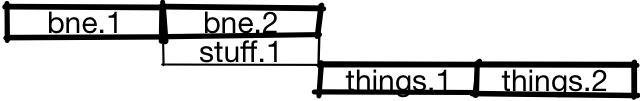
In this case, the processor predicts that the branch will not be busy, and begins the execution of the first half of the
stuff , while simultaneously ending the execution of the second half of the branch. If the prediction is correct, the CPU will execute the second half of the stuff and can start executing one more instruction, working with the second half of the stuff , as we saw in the first pipeline diagram.If the prediction is erroneous, then after completion of the execution of the branch, the CPU will discard the results of
stuff.1 and will start executing the correct instructions instead of the incorrect ones. Since, in the absence of transition prediction, we would stop the processor and do not execute any instructions, we do not lose anything in such a situation (at least at the approximation level with which we consider the situation).What is the performance impact? To evaluate it, you need to simulate performance and load. For this lecture, we take a caricature model of a conveyor CPU, where non-branching is worked out in approximately one instruction per cycle, unpredicted or incorrectly predicted transitions take 20 cycles, and correctly predicted transitions take one cycle.
If we take the most popular benchmark for integer loads on the SPECint "workstation", then the distribution can be 20% of branches and 80% of other operations. Without a prediction of transitions, we expect that the “average” instruction will take
branch_pct * 1 + non_branch_pct * 20 = 0.8 * 1 + 0.2 * 20 = 0.8 + 4 = 4.8 cycles. With an ideal 100% accurate prediction of transitions, the average instruction will take 0.8 * 1 + 0.2 * 1 = 1 cycle, which means acceleration 4.8 times! In other words, if we have a pipeline with a “fine” of 20 cycles for an unpredictable transition, then we get almost fivefold costs compared to the ideal pipeline, only due to branch prediction.See what you can do about it. Let's start with the simplest things, and gradually develop a better solution.
Take all the transitions
Instead of random predictions, we can look at all the branches of the execution of all programs. In this case, we will see that taken and unmarked branches are not equally balanced - the branches taken are much more than the uncivilized ones. One of the reasons are loop branches that are often executed.
If we predict the taking of each branch, then we can reach the level of prediction accuracy of 70%, so we will only pay for incorrectly predicted 30% of transitions, which reduces the cost of the average instruction to
(0.8 + 0.7 * 0.2) * 1 + 0.3 * 0.2 * 20 = 0.94 + 1.2. = 2.14 (0.8 + 0.7 * 0.2) * 1 + 0.3 * 0.2 * 20 = 0.94 + 1.2. = 2.14 . If we compare the mandatory prediction of all transitions with the lack of prediction and the ideal prediction, then the mandatory prediction plays most of the advantages of the ideal prediction, although this is a very simple algorithm.We take transitions back, we do not take forward transitions (BTFNT)
Predicting the taking of all branches works well for cycles, but not for other branches. If you look at the percentage of transitions carried forward in the program or back in the program (returning to the previous code), we will see that the transitions are performed more often than the transitions forward. Therefore, you can try a predictor that predicts taking all transitions back and not taking all transitions forward (BTFNT, backwards taken forwards not taken). If we implement this scheme at the hardware level, the compilers will adapt to us and begin to organize the code so that the branches with the greatest chances of execution become transitions back, and the branches with the least chances of execution become transitions forward.
If you do this, you can achieve prediction accuracy of about 80%, which reduces the cost of executing instructions to
(0.8 + 0.8 * 0.2) * 1 + 0.2 * 0.2 * 20 = 0.96 + 0.8 = 1.76 cycles.Who uses:
- PPC 601 (1993): also uses compiler tips in the form of generated transitions.
- PPC 603
One bit
So far, we have considered schemes that do not save any state, that is, such schemes, where the predictor ignores the program execution history. In the literature, they are called static transition prediction methods. Their advantage is simplicity, but they do poorly with predicting transitions that change over time. Here is an example of such a transition:
if (flag) { // things } During the execution of the program at one stage, the flag can be set and the transition is made, and at another stage there is no flag and the transition does not occur. Static methods cannot predict branching like this well, so consider dynamic methods, where the prediction may vary depending on the execution history of the program.
One of the simplest things is to predict on the basis of the last result, that is, to predict the transition if it took place the last time, and vice versa.
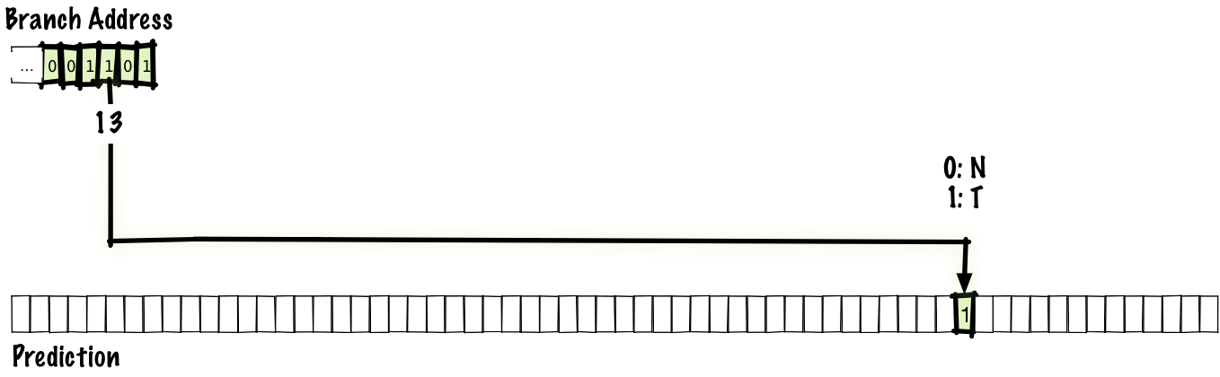
Since assigning a bit to each transition is too much for reasonable storage, we will make a table for a certain number of transitions that have taken place recently. For this lecture, assume that the absence of a transition corresponds to 0, and the capture of a branch is 1.
In our case, so that everything fits in the illustration, take a table with 64 entries. This number of records allows us to index the table with 6 bits, so that we use the lower 6 bits of the jump address. After the transition is completed, we update the state in the prediction table (highlighted below), and the next time in the index we use the already updated state.
Perhaps there will be an overlap and two branches from different places will point to the same address. The scheme is not perfect, but it is a compromise between the speed of the table and its size.
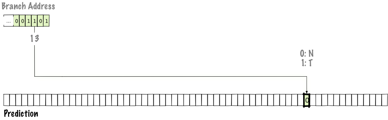
If you use a one-bit scheme, then we can achieve an accuracy of 85%, which corresponds to an average
(0.8 + 0.85 * 0.2) * 1 + 0.15 * 0.2 * 20 = 0.97 + 0.6 = 1.57 cycles per instruction.Who uses:
- DEC EV4 (1992)
- MIPS R8000 (1994)
Two bits
A one-bit scheme works well for templates of the form
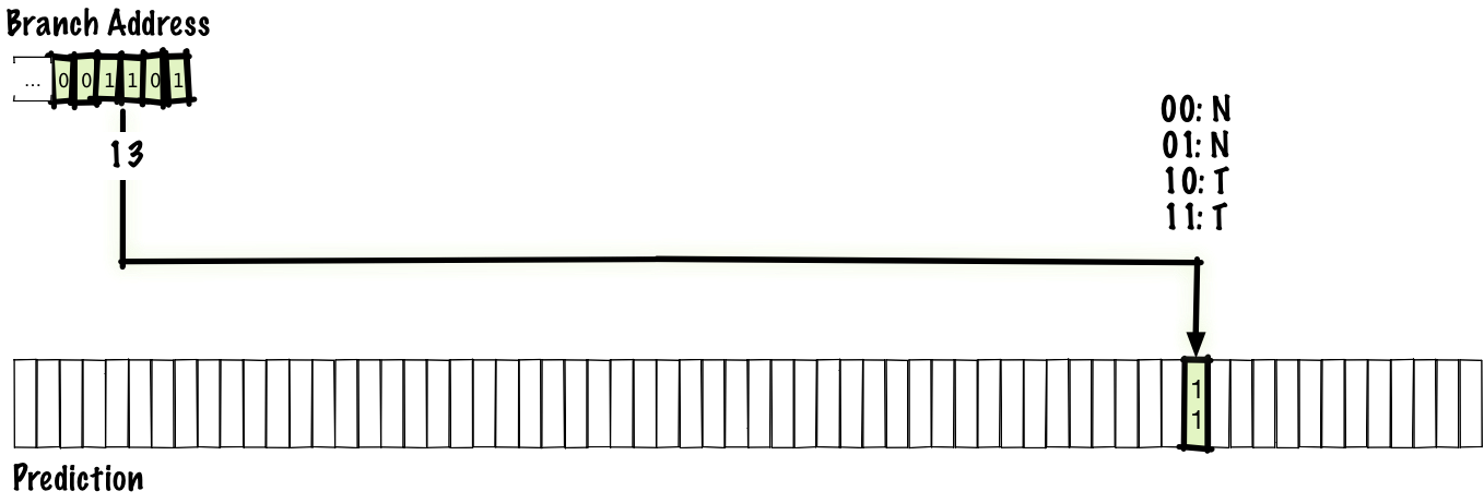
TTTTTTTT… or NNNNNNN… , but will give incorrect predictions for the branch flow, where most transitions occur, but one of them does not occur, ...TTTNTTT... This can be corrected by adding a second bit to each address and introducing a counter that implements saturation arithmetic. For example, we will take a unit if the transition did not take place, and add a unit if it took place. The binary results will be as follows:00: predict Not
01: predict Not
10: predict Taken
11: predict TakenThe “saturating” part of the counter means that if we count to 00, then we remain at this value. In the same way, if we count to 11, then we stay on it. This scheme is identical to one bit, but instead of one bit in the prediction table, we use two bits.
Compared to a single-bit scheme, a two-bit scheme can have half the number of records at the same size and cost (if we take into account only the cost of storage, but do not take into account the cost of the counter logic). But even so, for any reasonable table size, a two-bit scheme provides better accuracy.
Despite its simplicity, the scheme works quite successfully, and we can expect an increase in accuracy in the two-bit predictor to about 90%, which corresponds to 1.38 cycles per instruction.
It seems logical to generalize the scheme for an n-bit counter with saturation, but it turns out that increasing the bit depth has almost no effect on accuracy. We did not discuss the price of the branch predictor, but the transition from two to three bits increases the size of the table by a factor of one and a half for insignificant gain. In most cases it is not worth it. The simplest and most common cases that we cannot predict well with a two-bit predictor are patterns like
NTNTNTNTNT... or NNTNNTNNT… , but switching to more bits won't improve the accuracy in these cases either!Who uses:
- LLNL S-1 (1977)
- CDC Cyber? (early 80s)
- Burroughs B4900 (1982): the state is stored in the stream of instructions; at the hardware level, the instruction is overwritten to update the transition state
- Intel Pentium (1993)
- PPC 604 (1994)
- DEC EV45 (1993)
- DEC EV5 (1995)
- PA 8000 (1996): actually implemented as a three-bit shift register with a majority of votes.
Two-Level Adaptive Global Transition Prediction (1991)
If you think about this code
for (int i = 0; i < 3; ++i) { // code here. } Then it generates a branch pattern like
TTTNTTTNTTTN...If we know the three previous branch results, then we can predict the fourth:
TTT:N
TTN:T
TNT:T
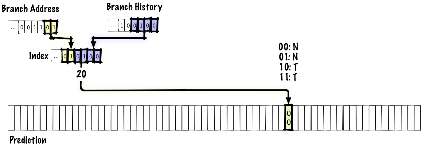
NTT:TThe previous schemes used the branch address to place the index in a table that indicated whether or not a transition was more likely depending on the program execution history. She says in which direction the branching will take place, but she is not able to guess that we are in the middle of a repeating pattern. To fix this, we will keep the history of most recent transitions, as well as a table of predictions.
In this example, we associate the four bits of the transition history with two bits of the transition address to place the index in the prediction table. As before, the source of the prediction is a two-bit counter with saturation. Here we do not want to use only the conversion history for the index. If you do this, then any two branches with the same history will refer to the same entry in the table. In a real predictor, we would probably have a larger table and more bits for the jump address, but we have to use a six-bit index to fit the table into the slide.
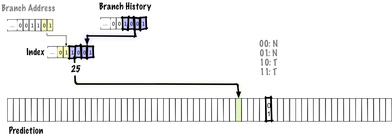
Below we see what value is updated during the transition.
Bold highlighted upgradeable parts. In this diagram, we shift the new bits of the transition history from right to left, updating the branch history. As the history is updated, the lower bits of the index in the prediction table are also updated, so the next time we encounter this branch, we use a different value from the table to predict the transition, unlike previous schemes, where the index was fixed in the transition address.
Since the global history is stored in this diagram, it will correctly predict patterns like
NTNTNTNT… in internal cycles, but it may not always correctly predict high-level branching, because global history is clogged with information from other branches. However, the trade-off here is that it is cheaper to keep global history than a table of local stories. In addition, the use of a global history allows you to correctly predict correlated branches. For example, we might have something like this: if x > 0: x -= 1 if y > 0: y -= 1 if x * y > 0: foo() If there is a transition along the first or second branch, the third one will definitely remain untapped.
With this scheme, we can achieve an accuracy of 93%, which corresponds to 1.27 cycles per instruction.
Who uses:
- Pentium MMX (1996): 4-Bit Global Transition History
Two-level adaptive local transition prediction (1992)
As mentioned above, the global history scheme has the problem that the history of local branches is clogged by other branches.
Good local predictions can be achieved by storing the history of local branches separately.
Instead of storing a single global history, we save a table of local histories, indexed by the address of the transition. Such a scheme is identical to the global scheme that we have just considered, with the exception of storing the histories of several branches. You can imagine a global history as a special case of a local history, where the number of stored stories is 1.
With this scheme, we can achieve an accuracy of 94%, which corresponds to 1.23 cycles per instruction
Who uses:
- Pentium Pro (1996): 4-bit history of local branching, the lower bits are used for the index . Please note that this issue is debatable, and Andrew Fogh states that PPro and subsequent processors use 4-bit global history.
- Pentium II (1997): the same as in PPro
- Pentium III (1999): the same as in PPro
gshare
In the global two-tier scheme, you have to compromise: in the fixed-size prediction table, the bits must match either the transition history or the transition address. We would like to allocate more bits for the transition history, because this will allow us to track the correlations at a greater distance, as well as to track more complex patterns. But we also want to give more bits under the address to avoid mutual interference between unrelated branches.
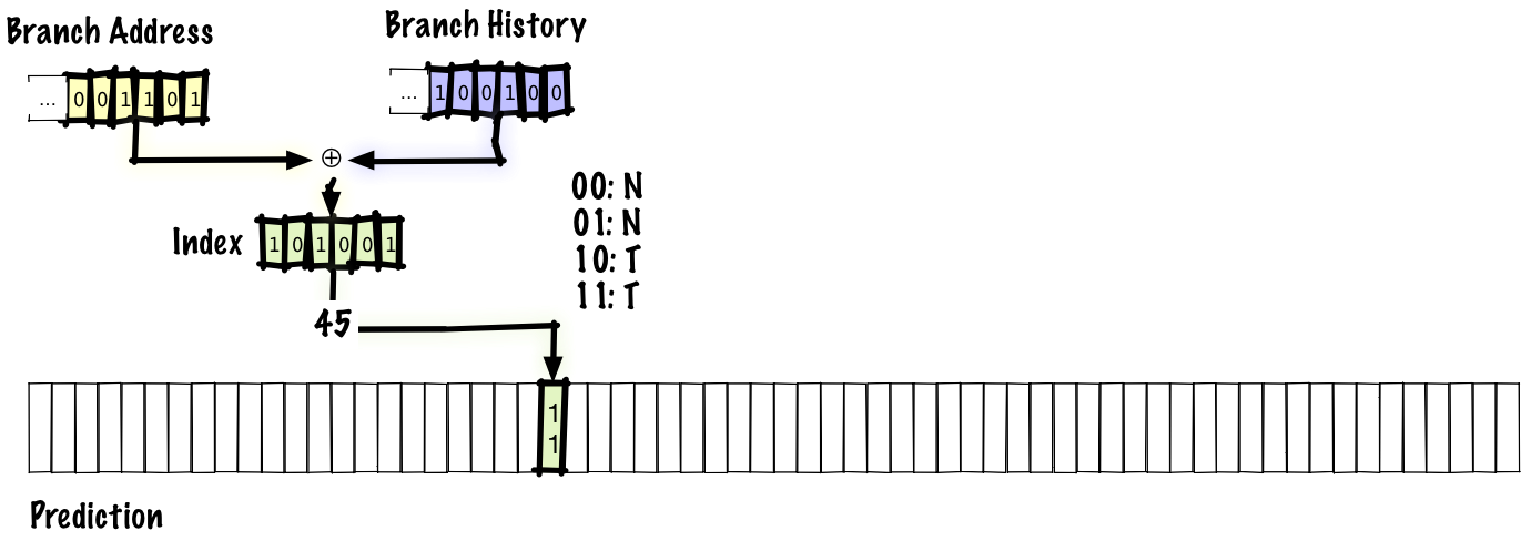
You can try to solve both problems by applying simultaneous hashing, and not the linkage of the transition history and the address of the transition. This is one of the simplest and most reasonable things we can do, and the first candidate for the role of the mechanism for this operation comes
xor . This two-level adaptive scheme where we use xor is called gshare .With this scheme, we can increase the accuracy to about 94%. This is the same accuracy as in the local scheme, but gshare does not need to store a large table of local stories.That is, we get the same accuracy at lower cost, which is a significant improvement.
Who uses:
- MIPS R12000 (1998): 2K records, 11 bits PC, 8 bits history
- UltraSPARC-3 (2001): 16K records, 14 bits PC, 12 bits history
agree (1997)
One of the reasons for incorrect prediction of transitions is interference between different branches that refer to the same address. There are many ways to reduce interference. In fact, in this lecture we look at the schemes of the 90s precisely because since then a large number of noise suppression schemes have been proposed, and there are too many of them to meet the half hour.
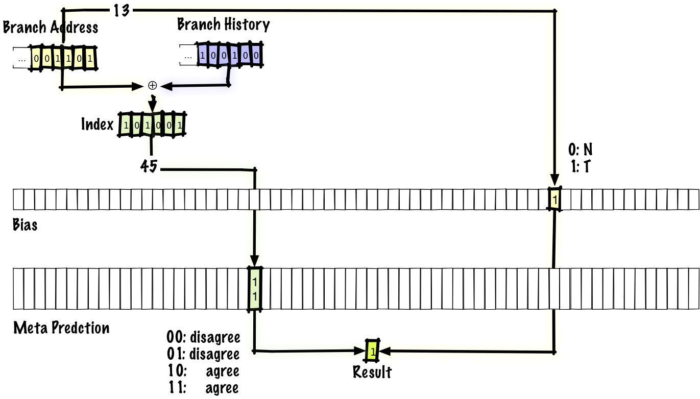
Let's look at one scheme that gives a general idea of how interference elimination may look like - this is the “agree” predictor. When a collision of two history-transition pairs occurs, the predictions either coincide or not. If they match, we call it neutral interference, and if not, then negative interference. The idea is that most of the branches have a strong bias in some way (that is, if we use a two-bit entry in the table of predictions, it is expected that most of the entries without interference most of the time will be equal to
00, or 11instead of 01, or10). For each transition in the program, we will store one bit, which we call “bias”. Instead of storing absolute transition predictions, the table will store information about whether or not the prediction matches the “bias” bit.If you look at how this works, then the predictor is identical to the gshare predictor, with the exception of the change we made - the prediction now looks like agree / disagree (agree or disagree), not taken / not taken (transition made or not implemented) , and we have the “bias” bit, which is indexed at the jump address, which gives us the material to make an agree / disagree decision. The authors of the original scientific article suggest using “bias” directly, but other experts have put forward the idea of defining “bias” by optimization based on profiling (essentially, when a working program sends data back to the compiler).
Notice that if we make the transition and then go back to the same branch, we will use the same bit “bias” because it is indexed by the transition address, but we will use another entry in the prediction table because it is indexed at the same time and the address of the transition, and the history of transitions.
If it seems strange to you that such a change matters, consider it with a specific example. Let's say we have two branches, branch A, on which the transition occurs with a probability of 90%, and branch B, on which the transition occurs with a probability of 10%. If we assume that the probabilities of transitions for each branch are independent of each other, then the probability of a disagree decision and negative interference is
P(A taken) * P(B not taken) + P(A not taken) + P(B taken) = (0.9 * 0.9) + (0.1 * 0.1) = 0.82.If we use the agree scheme, we can repeat this calculation, but the probability of a disagree decision making for the two branches and negative interference is
P(A agree) * P(B disagree) + P(A disagree) * P(B agree) = P(A taken) * P(B taken) + P(A not taken) * P(B taken) = (0.9 * 0.1) + (0.1 * 0.9) = 0.18. In other words, in order for destructive interference to appear, one of the branches must disagree with “bias”. By definition, if we correctly identified this bit, then the probability of this event cannot be large.With this scheme, we can achieve an accuracy of 95%, which corresponds to 1.19 cycles per instruction.
Who uses:
- PA-RISC 8700 (2001)
Hybrid (1993)
As we have seen, local predictors can well predict some types of branching (for example, built-in loops), and global predictors do well with other types (for example, with some correlated branches). You can try to combine the advantages of both predictors and get a meta-predictor that predicts whether to use a local or global predictor. A simple way is to use the same scheme for a meta-predictor as in the above-described two-bit predictor, but instead of a prediction,
takenor not takenit predicts a local or global predictor.Also, as there are many schemes for eliminating interference, one of which is the aforementioned agree scheme, there are also many hybrid schemes. We can use any two predictors, not only local and global, and the number of predictors is even more than two.
If we use global and local predictors, we can achieve an accuracy of 96%, which corresponds to a 1.15 cycle per instruction.
Who uses:
- DEC EV6 (1998): combination of local (1k records, 10 bits of history, 3 bits per counter) and global (4k records, 12 bits of history, 2 bits per counter) predictors
- IBM POWER4 (2001): local (16k records) and gshare (16k records, 11 bits of history, xor with a jump address, 16k selector table)
- IBM POWER5 (2004): a combination of bimodal (not covered here) and two-level adaptive predictors
- IBM POWER7 (2010)
What we missed
In this lecture, we have not talked about many things. As you might expect, the volume of the leaked material is much larger than the one we told you about. I will briefly mention some of the missing topics with links, so you can read about them if you want to know more.
One important thing we didn’t talk about was how to predict the destination of the transition . Note that this needs to be done even for some unconditional transitions (that is, for transitions that do not need special prediction, because they occur in any case), because (some) unconditional transitions have unknown goals .
Predicting the goal of a transition is so costly that some early CPUs had a transition prediction policy “to always predict no transition”, because the target address of the transition is not needed if there is no transition! Constant prediction of the absence of transitions has low accuracy, but it is still higher than if you do not make predictions at all.
Among the predictors with reduced interference, which we have not discussed, bi-mode , gskew and YAGS. Briefly, bi-mode is similar to agree in trying to split transitions by direction, but it uses a different mechanism: we maintain several prediction tables, and the third predictor uses the transition address to predict which table to use for a particular transition combination. and transition history. Bi-mode seems to be more successful than agree, as it has gained wider use. In the case of gksew, we maintain at least three prediction tables and separate hashes for indexing each table. The idea is that if two transitions overlap each other in the index, then this only happens in one table, so that we can vote and the result from the other two tables overlap the potentially bad result from the overlapping table. I do not know how to very briefly describe the scheme YAGS :-).
Since we did not talk about speed (delay), we did not talk about such a prediction strategy as using a small / fast predictor, the result of which can be covered by a slower and more accurate predictor.
Some modern CPUs have completely different conversion predictors; AMD Zen (2017) and AMD Bulldozer (2011) processors seem to use perceptron transition predictors . Perceptrons are single-level neural networks.
Allegedly , the Intel Haswell processor (2013) uses a variation of the TAGE predictor. TAGE means tagged geometric (TAgged Geometric) predictor with history size. If we study the predictors described by us and look at the actual execution of programs — which transitions are predicted incorrectly there, then there is one big class among them: these are transitions that need a big story. A significant number of transitions require dozens or hundreds of bits of history, and some even need more than a thousand bits of conversion history. If we have a single predictor or even a hybrid one that combines several different predictors, it will be inefficient to store a thousand bits of history, since this reduces the quality of predictions for transitions that need a relatively small history (especially in relation to price), and most of such transitions. One of the ideas behind the TAGE predictor is thatto keep the geometric lengths of the story sizes, and then each transition will use the corresponding story. This is an explanation of a part of GE in the abbreviation. The TA part means that the transitions are tagged. We did not discuss this mechanism; the predictor uses it to determine which story corresponds to which transitions.
In modern CPUs, specialized predictors are often used. For example, the cycle predictor can accurately predict transitions in cycles where the general transition predictor is not able to store a reasonable history size for perfect prediction of each iteration of the cycle.
We didn’t talk at all about the trade-off between memory usage and better predictions. Changing the size of the table not only changes the effectiveness of the predictor, but also changes the balance of forces in which predictor is better compared to others.
We also did not talk at all about how different tasks affect the performance of predictors of different types. Their effectiveness depends not only on the size of the table, but also on which particular program is running.
We also discussed the cost of incorrectly predicting a transition as if it were a constant value, but this was not the case , and in this respect the cost of instructions without transitions is also very different, depending on the type of task being performed.
I tried to avoid confusing terminology where possible, so if you read the literature, there is a slightly different terminology.
Conclusion
We reviewed a number of classical predictors of transitions and very briefly discussed a couple of newer predictors. Some of the classic predictors we considered are still used in processors, and if I had an hour of time, not half an hour, we could discuss the most up-to-date predictors. I think many people have the idea that a processor is a mysterious and difficult to understand thing, but in my opinion, processors are actually easier to understand than software. I may not be objective, because I used to work with processors, but still it seems to me that this is not my bias, but this is something fundamental.
If you think about the complexity of the software, then the only limiting factor of this complexity will be your imagination. If you can imagine something in such detailed detail that it can be recorded, then you can do it. Of course, in some cases the limiting factor is something more practical (for example, the performance of large-scale applications), but I think most of us spend most of the time writing programs, where the limiting factor is the ability to create and manage complexity.
The hardware is noticeably different here, because there are forces that oppose complexity. Every piece of iron you implement costs money, so you want to use a minimum of equipment. In addition, for most iron, performance is important (whether it is absolute performance or productivity per dollar, or per watt, or other resource), and the increase in complexity slows down the iron, which limits productivity. Today you can buy a serial CPU for $ 300, which accelerates to 5 GHz. At 5 GHz, one unit of work is performed in one fifth of a nanosecond. For information, light travels about 30 centimeters per nanosecond. Another deterrent is that people get very upset if the CPU doesn't work perfectly all the time. Although processors have bugs, the number of bugs is much less than in almost any software, that is, the standards for checking / testing them are much higher. Increasing complexity makes testing and verification difficult. Since processors adhere to a higher standard of accuracy than most software , increasing the complexity adds too much testing / testing burden for the CPU. Thus, the same complication is much more expensive for hardware than for software, even without taking into account other factors that we discussed.
A side effect of these factors that counteract the complexity of the chip is that each “high-level” function of a general-purpose processor is usually fairly conceptually simple to describe in half an hour or an hour lecture. Processors are simpler than many programmers think! By the way, I said “high-level” to exclude all sorts of things like devices of transistors and circuitry, for understanding of which a certain low-level background is needed (physics or electronics).
Source: https://habr.com/ru/post/337000/
All Articles