Simple models of economic dynamics in Python
Introduction
In my publications [1,2], economic problems were considered in statics without regard to time. In the tasks of optimization of economic dynamics, changes in economic parameters and their interrelations in time are analyzed. In models of economic dynamics, time can be considered as a discrete change in jumps, for example, over a year. Difference equations are used to describe such processes. With a continuous change in time, differential equations are used to describe the parameters of the model.
Formulation of the problem
For the first acquaintance with models of economic dynamics, it suffices to consider two typical models. This is the cobweb model and the Kaldor model and in which the two mentioned approaches to the description of economic dynamics are implemented.
Spider model of economic dynamics [3]
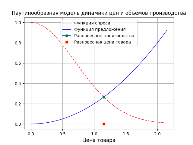
The model allows to investigate the stability of prices and production volumes in the market described by the demand and supply curves of a certain product. The demand function S (p) characterizes the dependence of the volume of demand for goods on the price p of the goods in a given period i. The supply function D (p) characterizes the volume of supply of goods depending on the price of goods. The equilibrium price p, of the market is determined by the equality of supply and demand S (p) = D (p).
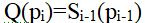
The manufacturer determines the volume of the offered goods on the basis of demand and prices for the goods established in the previous period - i-1.
')
To solve this equation, we define the volume in the initial period Q0 and using the inverse function of the proposal, we determine the price of the product.
The volume of production in the next period of time is determined by the demand function
and so on.
If the supply and demand functions change, then price fluctuations will be determined only by the deviation of the price from the equilibrium one.
Listing the cobweb pattern
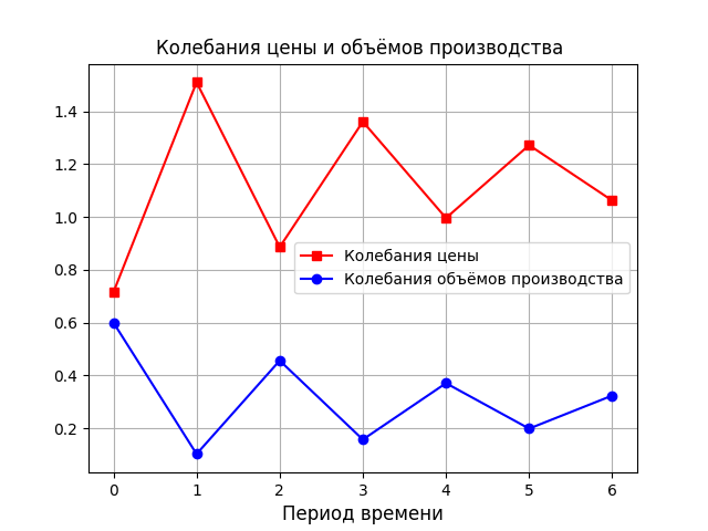
from scipy.optimize import * import numpy as np import matplotlib.pyplot as plt a=1;b=0.2# def fun_1(x,a): # return np.e**(-a*x**2) def fun_2(x,b): # return b*x**2 x0=round(fsolve(lambda x:fun_1(x,a)-fun_2(x,b),1)[0],3)# x=np.arange(0,x0+1,0.01) plt.figure() plt.title(' ', size=12) plt.xlabel(' ', size=12) plt.plot(x, fun_1(x,a), 'r', linestyle ='--',linewidth = 1, label=' ') plt.plot(x, fun_2(x,b), 'b', linestyle ='-' ,linewidth = 1, label=' ') plt.plot(x0, fun_2(x0,b), marker = 'o', markersize = 6, markerfacecolor = 'g', label=' ' ) plt.plot(x0, 0, marker = 's', markersize = 6, markerfacecolor = 'r', label=' ' ) plt.legend(loc='best') plt.grid(True) q=[];p=[];x=[] q.append(0.6) p.append(round(fsolve(lambda x:fun_1(x,a)-q[0],1)[0],3)) for i in np.arange(0,7): x.append(i) if i!=0: q.append(fun_2(p[i-1],b)) p.append(round(fsolve(lambda x:fun_1(x,a)-q[i],1)[0],3)) plt.figure() plt.title(' ', size=12) plt.xlabel(' ', size=12) plt.plot(x, p, 'r', marker = 's', markersize = 6, markerfacecolor = 'r', label=' ') plt.plot(x, q, 'b', marker = 'o', markersize = 6, markerfacecolor = 'b', label=' ') plt.legend(loc='best') plt.grid(True) plt.show() The results of the program
Conclusion
By adjusting the constants a, b according to the statistics of the commodity market (such an analysis is well developed in scipy.stats), the spider-like model can be used to adjust production volumes.
Model Kaldor [4]
The model attempts to explain the cyclical nature of changes in economic activity by the savings factors S (y) and investment I (y), where y is the income. In the model, the volume of savings and investments are not linear, but logistic (S-shaped) functions.
Kaldor Model Listing
from scipy.optimize import * from scipy.misc import derivative import numpy as np import matplotlib.pyplot as plt c=2.2;a=-0.9;h=0.1 def f(x): return 3*x-2*c*(a+x)**3+2*a**3-1.5 def s(x): return c*(a+x)**3-a**3+2 def l(x): return 3*xc*(a+x)**3+a**3+0.5 rx=[];ry=[];dy=[];dz=[] for i in np.arange(0,3): x=round(fsolve(lambda x:f(x),i)[0],3) z=derivative(f, x, dx=1e-6) rx.append(x) ry.append(s(x)) dz.append(z) x=[i*h for i in np.arange(0,18)] z=[s(i*h) for i in np.arange(0,18)] v=[l(i*h) for i in np.arange(0,18)] plt.figure() plt.title(' ', size=12) plt.xlabel('', size=12) plt.plot(x, z, 'r', linestyle ='--',linewidth = 2, label=' -s(x)') plt.plot(x, v, 'b', linestyle ='-' ,linewidth = 2, label=' -l(x)') plt.plot(rx[0], ry[0], marker = 's', markersize = 6, label=' y1 - df/dx<0,df/dx= '+ str(round(dz[0],3))) plt.plot(rx[1], ry[1], marker = 'o', markersize = 6, label=' y2 - df/dx>0,df/dx='+ str(round(dz[1],3))) plt.plot(rx[2], ry[2], marker = 's', markersize = 6, label=' y3 - df/dx<0,df/dx= '+ str(round(dz[2],3))) plt.legend(loc='best') plt.grid(True) T=4;N=50; h=T/N y=[];y.append(1.2) z=[];z.append(0.987) u=[];u.append(0.5) x=[ i*h for i in np.arange(0,N+2)] for i in np.arange(1,N+2): y.append(y[i-1]+h*f(y[i-1])) for i in np.arange(1,N+2): z.append(z[i-1]+h*f(z[i-1])) for i in np.arange(1,N+2): u.append(u[i-1]+h*f(u[i-1])) y1= [rx[0] for i in np.arange(0,N+2)] y3= [rx[2] for i in np.arange(0,N+2)] y2= [rx[1] for i in np.arange(0,N+2)] plt.figure() plt.title(' \n ', size=12) plt.plot(x, y,linewidth = 2, label=' f(x0)=1.2') plt.plot(x, z,linewidth = 2, label='f(x0)=0.987') plt.plot(x, u,linewidth = 2, label=' f(x0)=0.5') plt.plot(x, y1,linewidth = 1, label=' y1') plt.plot(x, y3,linewidth = 1, label=' y3') plt.plot(x, y2,linewidth = 1, label='y2') plt.legend(loc='best') plt.grid(True) plt.show() The result of the program is the dynamics of savings and investments.
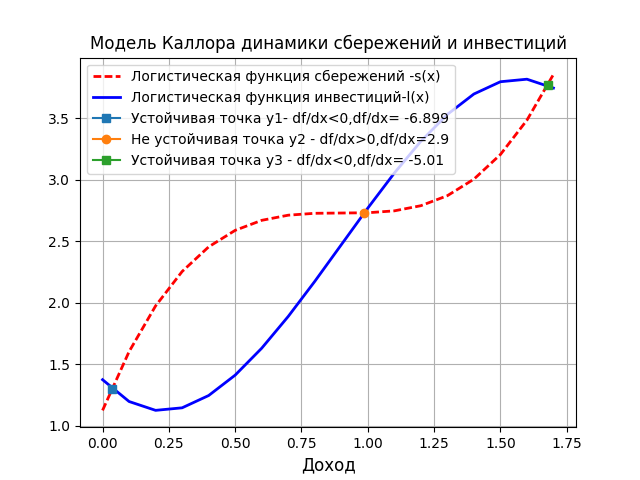
Equilibrium is achieved under the condition S (y) = 1 (y). There are three such points on the graph. There are only two stable points y1 and y3, because the derivative of the function f (y) = I (y) - S (y) in them is negative.
The change in income in such a system can be represented as a differential equation dy / dt = f (y) with initial conditions y (0) = y0.
The result of the program is an integrated income under various initial conditions.
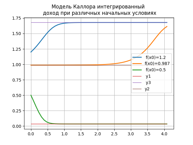
When the amount of income corresponds to one of the equilibrium states, it can be maintained indefinitely. However, changes in the economic situation for unstable equilibrium, for example, at the point y2, will lead to a transition to one of the stable points y1 or y3, depending on moving to the left or right from the equilibrium position. For stable points with small deviations from the equilibrium position, a return to the same state will occur. This is true with constant investment and savings functions. Periodic changes in business activity will lead to the deformation of these functions, which explains the cyclical nature of economic development and demonstrates the above graph.
Conclusion
By adjusting the constants for and with the savings and investment functions using statistical data, using the Callora model, one can get information to support management decisions.
Thank you all for your attention!
Links
Source: https://habr.com/ru/post/336946/
All Articles