Create your own physical 2D engine. Part 1: fundamentals and resolution of impulses of force

You can start creating your own physics engine for various reasons: firstly, to master and assimilate new knowledge in mathematics, physics and programming; secondly, its own physics engine can handle any technical effects that its author can create. In this introductory article I will explain how to create your own physics engine from scratch.

Physics gives the player great opportunities to dive into the game. I think that mastering the physics engine will be a very useful skill for any programmer. For a deeper understanding of the internal work of the engine, you can make any optimizations and specialized features at any time.
')
In this part of the tutorial we will cover the following topics:

Simple collision detection
Generating simple manifolds
Power impulse resolution

Here is a small demo:

Note: even though this tutorial is written in C ++, you can use the same techniques and concepts in almost any game development environment.

Required knowledge

Understanding this article requires a good knowledge of mathematics and geometry, and to a much lesser extent directly programming. In particular, you will need the following:

Basic understanding of the basics of vector mathematics
The ability to perform algebraic calculations

Collision detection

There are enough articles and tutorials on collision recognition on the Internet, so I will not discuss this topic in detail.

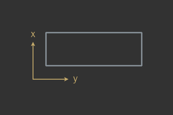
The bounding box aligned with the axes

A bounding rectangle aligned with the axes (Axis Aligned Bounding Box, AABB) is a rectangle whose four axes are aligned with the coordinate system in which it is located. This means that the rectangle cannot rotate and is always at a 90 degree angle (usually aligned with the screen). It is usually called the “bounding box” because AABB is used to restrict other, more complex shapes.

An example AABB

Example AABB.

Complicated AABBs can be used as a simple test to see if more complex shapes can intersect within an AABB. However, in the case of most games, AABB is used as a fundamental form and in fact does not limit anything. The structure of AABB is very important. There are several ways to set AABB, here is my favorite:

struct AABB { Vec2 min; Vec2 max; };

This form allows you to specify AABB with two points. The point min denotes the lower bounds in the x and y axes, and max denotes the upper bounds - in other words, they denote the upper left and lower right corners. To determine whether two AABBs intersect, a basic understanding of the separation axis theorem (Separating Axis Theorem, SAT) is necessary.

Here's a quick check taken from Krister Erickson's Real-Time Collision Detection site, which uses SAT:

 bool AABBvsAABB( AABB a, AABB b ) { //   ,      if(a.max.x < b.min.x or a.min.x > b.max.x) return false if(a.max.y < b.min.y or a.min.y > b.max.y) return false //    ,         return true }

Circumference

The circle is given by radius and point. Here is what the structure of the circle might look like:

 struct Circle { float radius Vec position };

Checking the intersection of two circles is very simple: take the radii of two circles and add them, then check whether this sum is greater than the distance between the two centers of the circles.

Important optimization, allowing to get rid of the square root operator:

 float Distance( Vec2 a, Vec2 b ) { return sqrt( (ax - bx)^2 + (ay - by)^2 ) } bool CirclevsCircleUnoptimized( Circle a, Circle b ) { float r = a.radius + b.radius return r < Distance( a.position, b.position ) } bool CirclevsCircleOptimized( Circle a, Circle b ) { float r = a.radius + b.radius r *= r return r < (ax + bx)^2 + (ay + by)^2 }

In the general case, multiplication is a much less expensive operation than getting the square root of a value.

Power impulse resolution

Power impulse resolution is a specific type of collision resolution strategy. Collision resolution is an action in which two intersecting objects are taken and changed so that they no longer intersect.

In the general case, an object in a physical engine has three main degrees of freedom (in two dimensions): motion in the xy plane and rotation. In this article, we deliberately limited the rotation and use only AABB with circles, so the only degree of freedom that we will need to consider is movement in the xy plane.

In the process of resolving the detected collisions, we impose such restrictions on the movement so that the objects cannot cross each other. The main idea of the resolution of force impulses is to use a force impulse (instantaneous change in speed) to separate objects that have collisions. To do this, somehow you need to take into account the position and speed of each of the objects: we want large objects that intersect with small ones, in case of collision they move a little, and small objects fly away from them. We also want objects with infinite mass not to move at all.

Simple example of what resolution can achieve

Simple example of what resolution can achieve

A simple example of what can be achieved with the help of the impulse resolution of force.

To achieve this effect and at the same time to follow an intuitive understanding of how objects should behave, we use solid bodies and a bit of mathematics. A solid body is simply a form defined by the user (that is, you, the developer), which is clearly defined as non-deformable. Both AABB and the circles in this article are non-deformable, and will always be either AABB or a circle. All compression and stretching is prohibited.

Working with solids allows you to greatly simplify a bunch of calculations. That is why solids are often used in games, and therefore we use them in this article.

Objects collided - what next?

Suppose we found a collision of two bodies. How to separate them? We assume that collision detection provides us with two important characteristics:

Collision normal
Penetration depth

To apply the impulse of force to both objects and push them away from each other, we need to know in which direction and how far they should be pushed. The collision normal is the direction in which the force impulse is applied. The depth of penetration (along with some other parameters) determines how large the impulse of force used will be. This means that the only value that we need to calculate is the magnitude of the impulse of force.

Now let's take a closer look at how to calculate the magnitude of the impulse force. Let's start with two objects for which an intersection is found:

Equation 1

V^{a b} = v^{b} - v^{a}

$V ^ {ab} = v ^ b - v ^ a$

Note that to create a vector from position A to position B you need to do: endpoint - startpoint .

V^{a b}

$V ^ {ab}$ - this is the relative speed from A to B. This equation can be expressed relative to the collision normal

n

$n$ , that is, we want to know the relative speed from A to B along the collision normal direction:

Equation 2

V^{A B} c d o t n = (V^{B} - V^{A}) c d o t n

$V ^ {AB} \ cdot n = (V ^ B - V ^ A) \ cdot n$

Now we use scalar product . Scalar product is simply the sum of component-wise products:

Equation 3

V_{1} = b e g i n b m a t r i x x_{1} y_{1} e n d b m a t r i x, V_{2} = b e g i n b m a t r i x x_{2} y_{2} e n d b m a t r i x V_{1} c d o t V_{2} = x_{1} * x_{2} + y_{2} * y_{2}

$V_1 = \ begin {bmatrix} x_1 \\ y_1 \ end {bmatrix}, V_2 = \ begin {bmatrix} x_2 \\ y_2 \ end {bmatrix} \\ V_1 \ cdot V_2 = x_1 * x_2 + y_2 * y_2$

The next step will be the introduction of the concept of coefficient of elasticity . Resilience is a concept meaning elasticity. Each object in the physics engine will have elasticity, represented as a decimal value. However, when calculating the force impulse, only one decimal value will be used.

To select the desired elasticity (denoted as

e

$e$ , "Epsilon"), which meets the intuitively expected results, we should use the least elasticity involved:

 //    A  B e = min( A.restitution, B.restitution )

Having received

e

$e$ , we can substitute it into the equation for calculating the magnitude of the impulse force.

The Newtonian law of restoration reads as follows:

Equation 4

V^{'} = e * v

$V '= e * v$

All it says is that the speed after a collision is equal to the speed before it, multiplied by some constant. This constant is the "repulsion coefficient". Knowing this, it is easy to substitute the elasticity in our current equation:

Equation 5

V^{A B} c d o t n = - e * (V^{B} - V^{A}) c d o t n

$V ^ {AB} \ cdot n = -e * (V ^ B - V ^ A) \ cdot n$

Notice that a negative value appeared here. Notice how we introduced a negative sign here. According to the Newtonian law of recovery

V^{'}

$V '$ , the resultant vector after the repulsion, is really directed in the opposite direction from V. So how do you imagine the opposite directions in our equation? Enter a minus sign.

Now we need to express these speeds under the influence of a momentum of force. Here is a simple equation for changing the vector to a scalar impulse force.

j

$j$ in a certain direction

n

$n$ :

Equation 6

V^{'} = V + j * n

$V '= V + j * n$

I hope this equation is clear to you, because it is very important. We have a single vector

n

$n$ indicating the direction. We also have a scalar

j

$j$ denoting the length of the vector

n

$n$ . When summing the scaled vector

n

$n$ with

V

$V$ we get

V^{'}

$V '$ . It is simply the addition of two vectors, and we can use this small equation to apply the momentum of one vector to another.

Here we have yet to do a little work. Formally, the impulse of force is defined as the change of impulse. Impulse is * . Knowing this, we can express the impulse according to a formal definition like this:

Equation 7

I m p u l s e = m a s s * V e l o c i t y V e l o c i t y = f r a c I m p u l s e m a s s t h e r e f o r e V^{'} = V + f r a c j * n m a s s

$Impulse = mass * Velocity \\ Velocity = \ frac {Impulse} {mass} \ therefore V '= V + \ frac {j * n} {mass}$

Three points in the shape of a triangle (

t h e r e f o r e

$\ therefore$ ) can be read as “hence.” This designation is used to derive the truth from the preceding one.

We are moving well! However, we need to express the impulse of power through

j

$j$ regarding two different objects. During the collision of objects A and B, object A repels in the direction opposite to B:

Equation 8

V^{' A} = V^{A} + f r a c j * n m a s s^{A} V^{' B} = V^{B} - f r a c j * n m a s s^{B}

$V '^ A = V ^ A + \ frac {j * n} {mass ^ A} \\ V' ^ B = V ^ B - \ frac {j * n} {mass ^ B}$

These two equations repel A from B along a unit vector of direction

n

$n$ on the scalar of the impulse force (magnitude

n

$n$ )

j

$j$ .

All this is necessary for combining equations 8 and 5. The final equation will look something like this:

Equation 9

(V^{A} - V^{V} + f r a c j * n m a s s^{A} + f r a c j * n m a s s^{B}) * n = - e * (V^{B} - V^{A}) c d o t n t h e r e f o r e (V^{A} - V^{V} + f r a c j * n m a s s^{A} + f r a c j * n m a s s^{B}) * n + e * (V^{B} - V^{A}) c d o t n = 0

$(V ^ A - V ^ V + \ frac {j * n} {mass ^ A} + \ frac {j * n} {mass ^ B}) * n = -e * (V ^ B - V ^ A ) \ cdot n \\ \ therefore \\ (V ^ A - V ^ V + \ frac {j * n} {mass ^ A} + \ frac {j * n} {mass ^ B}) * n + e * (V ^ B - V ^ A) \ cdot n = 0$

If you remember, our initial goal was to isolate the magnitude, because we know the direction in which we need to resolve the collision (it is given by the recognition of collisions), and we just have to determine the magnitude in that direction. In our case, the unknown value

j

$j$ ; we need to highlight

j

$j$ and solve the equation for her.

Equation 10

(V^{B} - V^{A}) c d o t n + j * (f r a c j * n m a s s^{A} + f r a c j * n m a s s^{B}) * n + e * (V^{B} - V^{A}) c d o t n = 0 t h e r e f o r e (1 + e) ​ ​ ((V^{B} - V^{A}) c d o t n) + j * (f r a c j * n m a s s^{A} + f r a c j * n m a s s^{B}) * n = 0 t h e r e f o r e j = f r a c - (1 + e) ​ ​ ((V^{B} - V^{A}) c d o t n) f r a c 1 m a s s^{A} + f r a c 1 m a s s^{B}

$(V ^ B - V ^ A) \ cdot n + j * (\ frac {j * n} {mass ^ A} + \ frac {j * n} {mass ^ B}) * n + e * (V ^ B - V ^ A) \ cdot n = 0 \\ \ therefore \\ (1 + e) ((V ^ B - V ^ A) \ cdot n) + j * (\ frac {j * n} {mass ^ A} + \ frac {j * n} {mass ^ B}) * n = 0 \\ \ therefore \\ j = \ frac {- (1 + e) ((V ^ B - V ^ A) \ cdot n)} {\ frac {1} {mass ^ A} + \ frac {1} {mass ^ B}}$

Wow, quite a lot of calculations! But that's all. It is important to understand that in the final form of equation 10 on the left we have

j

$j$ (value), and we already know everything on the right. This means that we can write a couple of lines of code to calculate the force impulse scalar.

j

$j$ . And this code is much more readable than mathematical writing!

 void ResolveCollision( Object A, Object B ) { //    Vec2 rv = B.velocity - A.velocity //       float velAlongNormal = DotProduct( rv, normal ) //   ,    if(velAlongNormal > 0) return; //   float e = min( A.restitution, B.restitution) //     float j = -(1 + e) * velAlongNormal j /= 1 / A.mass + 1 / B.mass //    Vec2 impulse = j * normal A.velocity -= 1 / A.mass * impulse B.velocity += 1 / B.mass * impulse }

In this sample code, two important aspects need to be noted. First, look at line 10, if(VelAlongNormal > 0) . This check is very important; it ensures that we resolve the collision only if the objects move towards each other.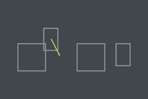

Two objects collide

The two objects have a collision, but the speed will separate them in the next frame. We do not allow this type of collision.

If objects move in opposite directions, we do nothing. Due to this, we will not allow collisions of those objects that do not actually collide. This is important for creating simulations that meet intuitive expectations about what should happen when objects interact.

Secondly, it is worth noting that the reverse mass is calculated without any reason several times. It is best to simply save the reverse mass inside each object and calculate it at the same time in advance:

 A.inv_mass = 1 / A.mass

In many physical engines, the raw mass is not actually stored. Often, physical engines store only the inverse of the mass. It just so happens that in most mathematical calculations the mass is used in the form of 1/ .

And the last thing to notice is that we must intelligently distribute our scalar impulse of force

j

$j$ on two objects. We want small objects to fly away from larger ones with a larger share

j

$j$ , and the speeds of large objects changed to a very small fraction

j

$j$ .

To do this, you can do the following:

 float mass_sum = A.mass + B.mass float ratio = A.mass / mass_sum A.velocity -= ratio * impulse ratio = B.mass / mass_sum B.velocity += ratio * impulse

It is important to realize that this code is similar to the above example of the ResolveCollision() function. As explained above, inverse masses are quite useful in a physics engine.

Sinking objects

If we use the already written code, the objects will collide and fly away from each other. This is great, but what happens if one of the objects has infinite mass? We will need a convenient way of setting in our simulation infinite mass.

I propose to use zero as infinite mass - however, if we try to calculate the inverse mass of an object with zero mass, we get the division by zero. To solve this problem when calculating the inverse mass can be as follows:

 if(A.mass == 0) A.inv_mass = 0 else A.inv_mass = 1 / A.mass

The value “zero” will lead to correct calculations when resolving impulses of force. It suits us. The problem of sinking objects arises when some object begins to "sink" in another due to gravity. Sometimes an object with low elasticity hits a wall with an infinite mass and begins to sink.

Such a drowning occurs due to floating-point computation errors. During each floating point calculation, a small error is added due to hardware limitations. (For details, see [Floating point error IEEE754] on Google.) Over time, this error accumulates into a positioning error, which causes objects to drown in each other.

To correct this positioning error, it is necessary to take it into account, so I will show you a method called “linear projection”. Linear projection onto a small percentage reduces the penetration of two objects into each other. It is performed after the application of a pulse of force. Correction is very simple: move each object along the collision normal

n

$n$ by percentage of penetration depth:

 void PositionalCorrection( Object A, Object B ) { const float percent = 0.2 //   20%  80% Vec2 correction = penetrationDepth / (A.inv_mass + B.inv_mass)) * percent * n A.position -= A.inv_mass * correction B.position += B.inv_mass * correction }

Note that we scale penetrationDepth to the total mass of the system. This will give us a position correction proportional to the mass. Small objects repel faster than heavy ones.

However, there is a small problem with this implementation: if we always resolve a positioning error, then objects will always tremble while they are on top of each other. To eliminate jitter, you need to set a small tolerance. We will only perform position adjustments if the penetration is above a certain arbitrary threshold, which we will call “slop”:

 void PositionalCorrection( Object A, Object B ) { const float percent = 0.2 //   20%  80% const float slop = 0.01 //   0.01  0.1 Vec2 correction = max( penetration - k_slop, 0.0f ) / (A.inv_mass + B.inv_mass)) * percent * n A.position -= A.inv_mass * correction B.position += B.inv_mass * correction }

This will allow objects to penetrate each other slightly without triggering a position correction.

Generating simple manifolds

The last thing we consider in this part of the article is the generation of a simple manifold. Diversity in mathematics is something like a “collection of points representing an area of space.” However, here by “diversity” I will understand a small object containing information about a collision between two objects.

This is what a standard manifold ad looks like:

 struct Manifold { Object *A; Object *B; float penetration; Vec2 normal; };

During collision recognition, it is necessary to calculate the penetration and normal of a collision. To determine this information, it is necessary to expand the original collision recognition algorithms from the beginning of the article.

Circle-circle

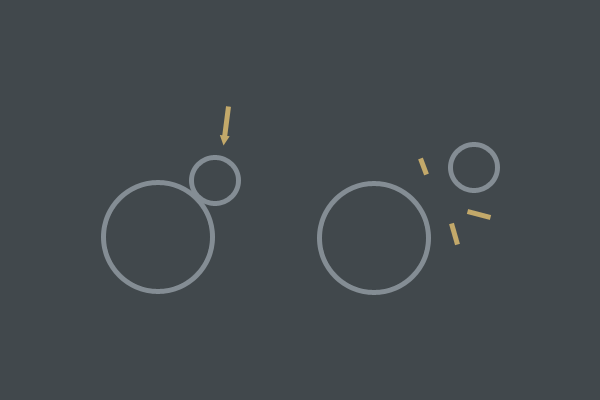
Let's start with the simplest collision algorithm: a circle-circle collision. This check is more trivial. Can you imagine what will be the direction of conflict resolution? This is a vector from circle A to circle B. It can be obtained by subtracting the position B from position A.

The depth of penetration is related to the radii of the circles and the distance between them. The overlap of circles can be calculated by subtracting from the sum of the radii of the distance to each of the objects.

Here is a complete example of a circle-circle collision manifold generation algorithm:

 bool CirclevsCircle( Manifold *m ) { //       Object *A = m->A; Object *B = m->B; //   A  B Vec2 n = B->pos - A->pos float r = A->radius + B->radius r *= r if(n.LengthSquared( ) > r) return false //    ,   float d = n.Length( ) //  sqrt //        if(d != 0) { //  -       m->penetration = r - d //  d,      sqrt  Length( ) //   A  B,     c->normal = t / d return true } //     else { //   ( )  c->penetration = A->radius c->normal = Vec( 1, 0 ) return true } }

Here it is worth noting the following: we do not perform square root calculations, so far we can do without it (if the objects have no collision), and we check whether the circles are at one point. If they are at one point, then the distance will be equal to zero and one should avoid dividing by zero when calculating t / d .

AABB-AABB

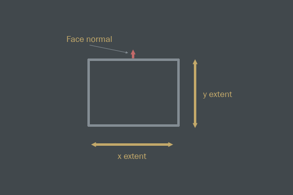
The AABB-AABB check is slightly more complex than a circle-circle. The collision normal will not be a vector from A to B, but will be normal to the edge. AABB is a rectangle with four edges. Each edge has a normal. This normal denotes a unit vector perpendicular to the edge.

Investigate the general equation of a line in 2D:

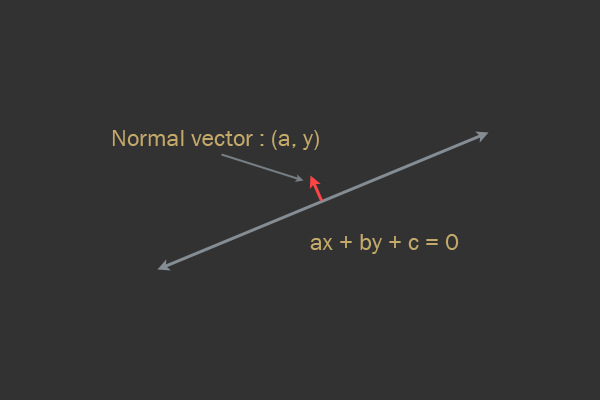
a x + b y + c = 0 n o r m a l = b e g i n b m a t r i x a b e n d b m a t r i x

$ax + by + c = 0 \\ normal = \ begin {bmatrix} a \\ b \ end {bmatrix}$

In the equation above, a and b are the normal vector to the straight line, and the vector (a, b) is considered normalized (the length of the vector is zero). The collision normal (the direction of collision resolution) will be directed toward one of the edge normals.

Do you know what is meant by c in the general equation of a straight line? c is the distance to the origin. As we will see in the next part of the article, this is very useful for checking on which side of the line there is a point.

All that is needed now is to determine which of the edges of one object collides with another object, after which we get the normal. However, sometimes several edges of two AABBs can intersect, for example, when crossing two corners. This means that we need to determine the axis of least penetration .

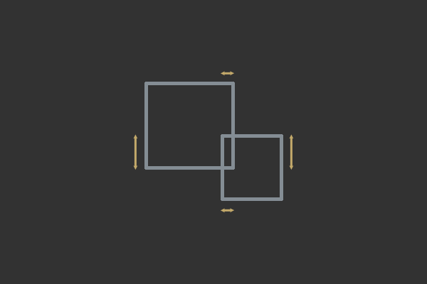
This should not be resolved along the x axis.

This should not be resolved along the x axis.

Two axes of penetration; the horizontal axis X is the axis of least penetration; therefore, this collision must be resolved along the X axis.

Here is the complete algorithm for generating the AABB-AABB manifold and collision recognition:

custom-physics-aabb-diagram

 bool AABBvsAABB( Manifold *m ) { //        Object *A = m->A Object *B = m->B //   A  B Vec2 n = B->pos - A->pos AABB abox = A->aabb AABB bbox = B->aabb //      x    float a_extent = (abox.max.x - abox.min.x) / 2 float b_extent = (bbox.max.x - bbox.min.x) / 2 //     x float x_overlap = a_extent + b_extent - abs( nx ) //  SAT   x if(x_overlap > 0) { //      y    float a_extent = (abox.max.y - abox.min.y) / 2 float b_extent = (bbox.max.y - bbox.min.y) / 2 //     y float y_overlap = a_extent + b_extent - abs( ny ) //  SAT   y if(y_overlap > 0) { // ,       if(x_overlap > y_overlap) { //    B, ,  n     A  B if(nx < 0) m->normal = Vec2( -1, 0 ) else m->normal = Vec2( 0, 0 ) m->penetration = x_overlap return true } else { //    B, ,  n     A  B if(ny < 0) m->normal = Vec2( 0, -1 ) else m->normal = Vec2( 0, 1 ) m->penetration = y_overlap return true } } } }

-AABB

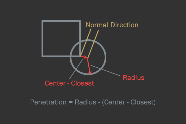
The last check I’ll review is the circle-AABB check. The idea here is to calculate the point AABB closest to the circle; thereafter, the check is simplified to something like a circle-circle check. After calculating the closest point and recognizing collisions, the normal will be the direction to the nearest point from the center of the circle. The depth of penetration is the difference between the distances to the point closest to the circle and the radius of the circle.

AABB to Circle intersection diagram

The intersection of the AABB-circle.

There is one tricky special case - if the center of the circle is inside the AABB, then you need to cut off the center of the circle to the nearest edge of the AABB and reflect the normal.

 bool AABBvsCircle( Manifold *m ) { //        Object *A = m->A Object *B = m->B //   A  B Vec2 n = B->pos - A->pos //    B  A Vec2 closest = n //       float x_extent = (A->aabb.max.x - A->aabb.min.x) / 2 float y_extent = (A->aabb.max.y - A->aabb.min.y) / 2 //    AABB closest.x = Clamp( -x_extent, x_extent, closest.x ) closest.y = Clamp( -y_extent, y_extent, closest.y ) bool inside = false //   AABB,       //    if(n == closest) { inside = true //    if(abs( nx ) > abs( ny )) { //     if(closest.x > 0) closest.x = x_extent else closest.x = -x_extent } //  y  else { //     if(closest.y > 0) closest.y = y_extent else closest.y = -y_extent } } Vec2 normal = n - closest real d = normal.LengthSquared( ) real r = B->radius //   ,       //     AABB if(d > r * r && !inside) return false //  sqrt,      d = sqrt( d ) //     AABB,      //    if(inside) { m->normal = -n m->penetration = r - d } else { m->normal = n m->penetration = r - d } return true }

Conclusion

I hope you now understand a bit more about physics simulation. This tutorial will be enough for you to start creating your own physics engine from scratch. In the next part, we will consider all the necessary extensions needed by the physics engine, namely:

Sorting and clipping contact pairs
Wide phase
Stratification
Integration
So you
Intersection of half spaces
Modularity (materials, mass and strength)

Source: https://habr.com/ru/post/336908/

All Articles