Heading "We read articles for you." August 2017

Hi, Habr! With this release, we begin a good tradition: every month there will be a set of reviews of some scientific articles from members of the Open Data Science community from the #article_essence channel. Want to get them before everyone else - join the ODS community!
Articles are selected either from personal interest, or because of the proximity to the ongoing competition. If you want to offer your article or you have any suggestions - just write in the comments and we will try to take everything into account in the future.
Articles for today:
- Fitting to Noise or Nothing At All: Machine Learning in Markets
- Learned in Translation: Contextualized Word Vectors
- Create Anime Characters with AI!
- LiveMaps: Converting Map Images into Interactive Maps
- Random Erasing Data Augmentation
- YellowFin and the Art of Momentum Tuning
- The devil is in the decoder
- Improving Deep Learning using Generic Data Augmentation
- Learning both Weights and Connections for Efficient Neural Networks
- Focal Loss for Dense Object Detection
- Borrowing Treasures from the Wealthy: Deep Transfer Learning through Selective Joint Fine-tuning
- Model-Agnostic Meta-Learning for Fast Networks
1. Fitting to Noise or Nothing At All: Machine Learning in Markets
Original article
Posted by: kt {at} ut {dot} ee
This is a review of an article in which diplomatic markets predict financial markets. The author of the post (hereinafter - ZHD) points to the following obvious nonsense of this and similar articles:
- Pulling the ears indicator accuracy method of taking the maximum of all experiments. The median, on the contrary, just corresponds to a random prediction.
- Boasting "good results" that are obtained on instruments that are not being traded at all (i.e., they have a constant price). In general, ZHD recommends comparing trading models not with a random predictor, but with a buy and hold strategy.
- The authors "simulate" their strategy, assuming the absence of commissions in transactions and the fact that any transaction can be executed at a price equal to the average between high and low in the last five minutes. Because of this, in simulations the best profit is obtained by the least liquid instruments (which in fact will not always sell at an average price in five minutes, so all profits are most likely “received” due to an unfair assumption about liquidity). In addition, the authors boast only a few "successful" models, keeping silent about everything that was simulated in the negative.
- The authors do not take into account the time of the stock exchanges (including face-to-face sessions for trading pits) and, according to ZHD, this is wrong.
2. Learned in Translation: Contextualized Word Vectors
→ Original article
→ Code
Posted by: kt {at} ut {dot} ee
Shuttle Learning in our time is a standard trick. Take the grid, trained on the rocks of the lapdogs from ImageNet, and fasten it somewhere to recognize the types of snot - this is already a standard program for all mamlevye diplornerov. In the context of text processing, transfer lerning is usually less deep and rests on the use of harvested word vectors such as Word2Vec, GloVe, etc.
The authors of the article propose to deepen the text transfer lerning to one level as follows:
- We will train the LSTM-based seq2seq model (of the type encoder + decoder hidden states) to translate, say, from English to German.
- Take from it only the encoder (it will be a simple LSTM type (Embedding (word_idxs)). This encoder can turn a sequence of words into an LSTM hidden states sequence. Since these hidden states are not taken by chance (their translation model uses in its attentions), then they will definitely have a useful signal.
- And that's all, now let's build any other text models that we will feed not only GloVe word vectors to the input, but also the corresponding LSTM hidden vectors glued to them from our translation encoder (we will call them Context Vectors, CoVe).
Next, the authors wind up some nontrivial model with biattention and maxout (apparently lost in their past work) and compare how it works in different tasks, if she feeds random embedding, GloVe, GloVe + CoVe, GloVe + CoVe + CharNGramEmbeddings at the entrance .
According to the results, the addition of CoVe seems to increase the accuracy of bare GloVe by about 1%. Sometimes the effect is less, sometimes negative, sometimes adding CharVGrams instead of CoVe works the same way or even better. In any case, the combination of GloVe + CoVe + CharNGrams works exactly better than all other methods.

In my opinion, due to the fact that the authors put a non-sickly model with an attentive on top of the embedding types being compared (GloVe vs CoVe), the measurement of the CoVe utility effect turned out to be overly noisy and not very convincing. I would prefer to see a more "laboratory" measurement.
3. Create Anime Characters with AI!
→ Original article
→ Site
Posted by: kt {at} ut {dot} ee
There is a site Getchu, which contains "profiles" of anime characters of various Japanese games with pictures and illustrations. These pictures can be downloaded.
To find the face in the picture, you can use some kind of tool "lbpcascade animeface". Thus, the authors received 42k anime faces, which they then revised with pens and threw out 4% of bad examples.
There is a certain ready-made CNN-model Illustration2Vec, which is able to recognize in anime pictures the properties like "smile", "hair color", and so on. The authors used it to remove the pictures and selected 34 tags of interest to them.
The authors stuffed it all into DRAGAN (Kodali et al, where this is different from the usual GAN, the authors do not go deep, apparently not fundamentally).
To be able to generate images with given attributes, the authors do as in ACGAN:
- Feed the generator vector attributes.
- They make the discriminator predict this vector.
- Additionally, the generator is fined in proportion to how discriminator did not guess the correct class.
Both the generator and the discriminator are rather confused convolutional SRResNets (the generator is 16-block, the discriminator is 10-block). The authors have removed the discriminator layers "since it wouldn’t be corrected for the computation of the gradient norm." I did not quite understand this problem, explain if you suddenly understand to whom.
Everything was trained by Adam with decreasing lr starting from 0.0002, it is not very clear how long.
For webapp authors have converted the network under WebDNN ( https://github.com/mil-tokyo/webdnn ) and therefore generate all the images directly in the browser on the client (!).
4. LiveMaps: Converting Map Images into Interactive Maps
→ Original article
→ Article - winner of Best Short Paper Awart SIGIR 2017
Posted by: zevsone
A fundamentally new system (LiveMaps) was proposed for analyzing map images and extracting the relevant viewport.
The system allows you to make annotations for images obtained using the search engine, allowing users to click on a link that opens an interactive map with the center in the location corresponding to the found image.
LiveMaps works in several tricks. First, it is checked whether the image is a map.
If yes, the system tries to determine the geolocation of this image. To determine the location, text and visual information extracted from the image is used. As a result, the system creates an interactive map displaying the geographic area calculated for the image.
Evaluation results on dataset locations with high rank show that the system is able to construct very accurate interactive maps, while achieving good coverage.
PS I did not expect to receive the best short paper award at such a venerable confe (121 short paper in this year's bidders, all the industry giants).
5. Random Erasing Data Augmentation
→ Original article
By: egor.v.panfilov {at} gmail {dot} com
The article is devoted to the study of one of the simplest methods of image augmentation - Random Erasing (in Russian, painting random rectangles).
The augmentation was parameterized with 4 parameters: (P_prob) the probability of applying a batch to each picture, (P_area) region size (area ratio), (P_aspect) aspect ratio of the region (aspect ratio), (P_value) filled with value: random / average on ImageNet / 0/255.

The authors assessed the impact of this augmentation method on 3 problems: (A) object classification, (B) object detection, © person re-identification.
(A) : 6 architectures were used, starting with AlexNet, ending with ResNeXt. Dataset - CIFAR10 / 100. The optimal value of the parameters: P_prob = 0.5, P_aspect = in a wide range, but preferably not 1 (square), P_area = 0.02-0.4 (2-40% of the image), P_value = random or average on ImageNet, for 0 and 255 the results are significantly worse . Compared with other methods and augmentation (random cropping, random flipping), and regularization (dropout, random noise): in order of decreasing efficiency - all together, random cropping, random flipping, random erasing. Drouput and random noise this method will be scattered. In general, the method is not the most powerful, but with optimal parameters it stably gives 1% accuracy (5.5% -> 4.5%). They also write that it increases the robustness of the classifier to the overlapping of objects: you-dont-say :.
(B) : Used Fast-RCNN at PASCAL VOC 2007 + 2012. We implemented 3 schemes: IRE (Image-aware Random Erasing, we also select the region for zero blind), ORE (Object-aware, we zero only parts of the bounding boxes), I + ORE (both there and there). There is no significant difference in mAP between these methods. Compared with pure Fast-RCNN, they give about 5% (67-> 71 on VOC07, 70-> 75 on VOC07 + 12), as much as A-Fast-RCNN . The optimal parameters are P_prob = 0.5, P_area = 0.02–0.2 (2–20%), P_aspect = 0.3–3.33 (from the lying to the standing bar).
(C) : ID-discim.Embedding (IDE), Triplet Net, and SVD-Net (all based on ResNet, pre-trained on ImageNet) on Market-1501 / DukeMTMC-reID / CUHK03 were used. On all models and datasets, augmentation stably gives at least 2% (up to 8%) for Rank @ 1, and at least 3% (up to 8%) for mAP. The parameters are the same as for (B).
In general, despite the simplicity of the method, the study and the article are quite neat and detailed (10 pages), with a bunch of graphs and tables. The Chinese were pleased, you will not say anything.
6. YellowFin and the Art of Momentum Tuning
→ Original article
→ Additional material about momentum
Posted by: Arech
I read it a long time ago, so it’s very, very superficial: after thoughtful smoking of the properties of the classic momentum (it’s also the momentum of Boris Polyak), on one-dimensional strictly convex quadratic purposes, the guys pulled out (or found someone?) Inequality connecting the coefficients of learning rate and momentum so that they fall into a “robust” region, which guarantees the fastest convergence of the SGD algorithm. Then they showed (?) That this assertion in principle can somehow be carried out for some nonconvex functions, at least in some of their local domains, which can be more or less approximated by a quadratic approximation. After that, they decided to file down their YellowFin tuner, which, on the basis of knowledge of the previous history of the gradient change, would approximate the surface functions of the error function necessary for inequality (gradient dispersion, some “generalized” surface curvature and the distance to the local minimum of the current point quadratic approximation) and, using these approximations would give the appropriate values for learning rate and momentum for use in SGD.
Also, having studied the issue of asynchronous (distributed) training of networks, the dudes proposed a generalization of their method (Closed-loop YellowFin), which takes into account that the real momentum in such conditions turns out to be more than planned.
We tested convolutional 110- and 164-layer ResNet on CIFAR10 and 100, respectively, and some LSTM on PTB, TS, and WSJ. The results are interesting (from x1.18 to x2.8 acceleration relative to Adam), but, as usual, there are questions to the experiment - rough selection of coefficients for the competencers, + emnip, only one run for each architecture, + only the results of the training set are shown ... In short, there is something to get to the bottom ...
Something like that, I hope, for the details, I did not strongly lie.
I was thinking to cut it to my libine, but I was firmly in trouble with Self-Normalizing Neural Networks (SELU + AlphaDropout), which I had taken up a little earlier and which turned out to be extremely useful to me, so until my hands reached it. I follow that thread in Lesagne ( https://github.com/Lasagne/Lasagne/issues/856 - a person has problems with reproducing results) and in general, I hope that there will be more information on reproducing their results. So if anyone tries, share chokak.
7. The Devil is in the Decoder
→ Original article
Posted by: ternaus
The question with which UpSampling is better for different architectures, where there is a Decoder, pulls the minds of many, especially those who are fighting for the fifth decimal place in the problems of segmentation, super resolution, colorization, depth, boundary detection.
The guys from Google and UCL got confused and wrote an article where they decided empirically to check who is better and find the logic in it.
Checked - it turned out that there is a difference, but the logic is not very visible.
For segmentation:
[1] Transposed Conv = Upsampling + Conv and which everyone furiously uses in Unet norms.
[2] throwing skiped connections, that is, the transformation SegNet => Unet reinforced concrete draws. This is intuitive, but there are tsiferki.
[3] It seems that Separable Transposed, which is Transposed, but with a smaller number of parameters for segmentation, works better. I wish the people in #proj_cars checked it.
[4] The ingenious Bilinear additive Upsampling, which they proposed, works something like [3] on segmentation. But this is also in the direction of the team from #proj_cars check
[5] They drop residual connections somewhere, which can also add something in theory, but where exactly it is not very clear, and it draws very uncertainly and not always.
For segmentation tasks, they use resnet 50 as a base and then add a decoder on top.
For the problem of instance boundary detection, they decided to choose a metric, in which less overfit to the markup algorithm + tsiferki get more.
That is, During the evaluation, predicted contour pixels within three from ground truth pixels are assumed to be correct . What immediately raises the question of how this all is transferred to the task, where each pixel is important. (Kostin is remembered here as a satellite trick for searching for fences with a thickness of one pixel and how people are fighting for + -1 pixel at the borders in the task about cars)
[6] For all networks that they train, weights use L2 regularization of about 0.0002
Karpaty, it seems, also said in his time that he always does this for a more stable convergence. (I need to try this, if someone does this and it gives something noticeable, it would be nice to tell about it in the trader)
Summary:
[1] The question about who and when they better raised, but did not answer.
[2] They suggested another method of doing upsampling, which works no worse than others.
[3] They confirmed that the skipped connection definitely helps, and the residual - depending on the phase of the moon.
We are waiting for a month about what the human GridSearch will say on #proj_cars.
8. Improving Deep Learning using Generic Data Augmentation
→ Original article
By: egor.v.panfilov {at} gmail {dot} com
Epigraph: Chinese laurels do not give rest to anyone, even on the black continent. Good computers, however, have not been delivered yet, but Ternaus ordered to write, "and here they continue."
The authors tried to conduct a benchmark of augmentation methods of images on the task of image classification, and to develop recommendations for their use for various cases. As a first approximation, these methods are divided into 2 categories: Generic (generally applicable) and Complex (using domain information / generative). This article only covers Generic.
All experiments in the article were conducted on Caltech-101 (101 class, 9144 images) using ZFNet (half of the informative part of the article on how best to train vanilla ZFNet). We trained 30 epochs using DL4j. Considered augmentation methods: (1) without augmentation, (2-4) geometric: horizontal flipping, rotating (-30deg and + 30deg), cropping (4 corner crops), (5-7) photometric: color jittering, edge enhacement (we add the result of the Sobel filter to the image), fancy PCA (we strengthen the principal components on the images).
Results: to baseline (top1 / top5: 48.1% / 64.5%) (a) flipping gives + 1/2%, but increases accuracy variation, (b) rotating gives + 2%, (c) cropping gives + 14% , ( d) color jittering + 1.5 / 2.5% , (de) edge enhancement and fancy PCA at + 1/2%. Those. among geometrical methods in front of cropping, among photometric - color jittering. In conclusion, the authors write that a significant improvement in accuracy with cropping augmentation may be due to the fact that data is 4 times as large as the original (it’s not fate to balance). From the positive - 5-fold cross-validation was not forgotten when assessing the accuracy of the models. Why these augmentation methods were chosen specifically among others (including the more popular ones) we will probably find out in the next article.
9. Learning both Weights and Connections for Efficient Neural Networks
→ Original article
By: egor.v.panfilov {at} gmail {dot} com
The article considers the problem of high resource consumption by modern DNN architectures (in particular, CNN). The most important scourge is access to dynamic memory. For example, the inference network with 1 billion links at 20 Hz consumes ~ 13W.
The authors propose a method of reducing the number of active neurons and connections in the network - prunning. It works as follows: (1) we train the network in full dataset, (2) we mask the connections with weights below a certain level, (3) we train the remaining connections in full dataset. Steps (2) and (3) can and should be repeated several times, since aggressive (for 1 approach) prunning shows slightly worse results (for AlexNet on ImageNet, for example, 5x versus 9x). Tricks: use L2-regularization of the scales, when training reduce the dropout, reduce the learning rate, prun and retrain CONV and FC layers separately, throw out dead (non-connected) neurons according to the results of step (2).
The experiments were carried out in Caffe with networks Lenet-300-100, Lenet-5 on MNIST, AlexNet, VGG-16 on ImageNet. On MNIST: they reduced the number of weights and FLOPs by 12 times , and also found that the prunning exhibits the property of the attention mechanism (it cuts more at the edges). On ImageNet : AlexNet was trained 75 hours and retrained 173 hours, VGG-16 pruned and retrained 5 times. On scales it was possible to squeeze 9 and 13 times respectively, according to FLOPs - 3.3 and 5 times . The profile of how connections are prung is interesting: the first CONV layer shrinks less than 2 times, the next CONV - 3 or more (up to 12), hidden FCs - 10-20 times, the last FC layer - 4 times.
In conclusion, the authors present the results of comparing various prunning methods (with L1-, L2-regularization, with and without additional training, separately for CONV, separately for FC). In short, there is laziness to prune, then you learn a network with L1, and you can just throw out half of the layers. If not laziness - only L2, prunit and retrain iteratively ~ 5 times. And finally, storing the scales in the form of sparse from the authors gave an overhead of ~ 16% - it is not that critical when you have a network 10 times smaller.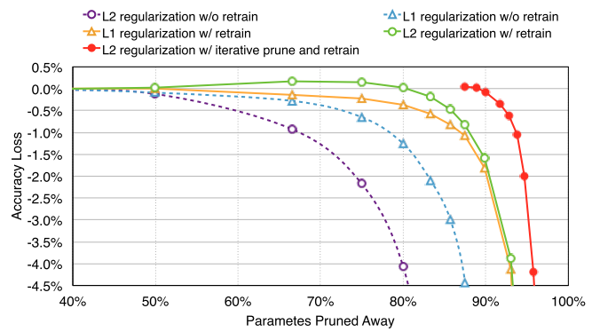
10. Focal Loss for Dense Object Detection
→ Original article
Posted by: kt {at} ut {dot} ee
As you know, the process of searching for models in machine learning rests on the optimization of a certain objective loss function. The simplest loss function is the percentage of errors at the training set, but it is difficult to optimize and the result is statistically bad, so in practice they use different surrogate losses: the square of the error, minus the logarithm of probability, the exponent of minus scoring, hinge loss, etc. All surrogate losses are monotonous functions that penalize errors the more, the greater the magnitude of the error. Any loss can be interpreted as the type of distribution of the target variable (for example, the square of the errors corresponds to the Gaussian distribution).
The authors found that the surrogate loss of the species
loss (p, y): = - (1-p) ^ gamma log (p) if y == 1 else -p ^ gamma log (1-p)
has never been used or published. Why do you need to use just such a loss, and not another one, and what is the meaning of the implied distribution, the authors do not know, but it seems to them funny, because there is an extra parameter gamma, with which you can, as it were, twist the fine value on "easy" examples. The authors called this feature "focal loss".
The authors selected one data set and one model-neural network on which, if the parameter values are adjusted, in the results plate one can see some positive effect from using such a loss instead of the usual cross-entropy (class-weighted). In fact, most of the article chews on the use of RetinaNet for the detection of objects, which are not strongly dependent on the choice of the loss function.
The article is required to read to all beginners on their way to the academy, because it perfectly illustrates how to write convincing-looking publications when there are no good ideas in my head.
Alternative opinion
Watch your hands: the dudes took one of the standard, rather complex datasets, which measure in detection, took a simple network without any special bells and whistles (which everyone else tried to squeeze as much as they could), attached their loss and got a single model result without a multskale and other tricks are higher than all others on this dataset, including all networks in one stage and more advanced two-stage ones. In order to make sure that it was a matter of the loss, and not something else, they tried other options that had previously been cool and fashionable techniques - balancing cross-entropy, OHEM and got results consistently higher on theirs. They twirled their parameters and found the option that works best and even tried a bit to explain why (there is a graph where it is clear that the gamma below 2 gives a fairly smooth distribution, and more than two it finishes very sharply (even with two there is almost a regiment, it is surprising that works)).
Of course, it was possible for them to start comparing 40 variants of networks, with a million variants of hyperparameters and on all known datasets, and even crossvalidation 10 times with 10 folds, but how long would that take and when would the publication be ready and how many different ones would there be ideas?
Everything is simple - one component was changed, the result was superior to SoTA on a particular dataset. Make sure that the result is caused by a change, and not by something else. Fin.
Alternative opinion
It is probably worth adding that if the article were positioned as a RetinaNet view, it would, in my opinion, look quite different. After all, it is built on the actual fact, mainly as an example of using RetinaNet. Why did they suddenly put an emphasis on the loss and a strange heading in it, I personally do not understand. There are still no objective measurements confirming the theses expressed about this loss.
Maybe, for example, RetinaNet is planned to be published in a more serious format and with a different order of authors, and this is simply a product of an off-site experiment, which was also decided to issue an extra publication because the student was working and well done. In this case, this is again an example of how to suck an extra article out of thin air.
In any case, I for myself can’t take out from this article the thesis promised in the title and text “screw such a loss everywhere and you will be happy”.
The thesis "RetinaNet works well for COCO (with any loss, moreover!)" I, at the same time, can quite well endure.
11. Borrowing Treasures from the Wealthy: Deep Transfer Learning through Selective Joint Fine-tuning
→ Original article
→ Code
Posted by: movchan74
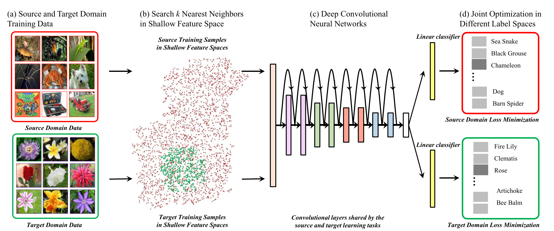
The authors focused on the problem of classifying images with a small dataset. In this case, a typical approach is the following: take the pre-trained CNN on ImageNet and retrain on your dataset (or even train only the classification fully connected layers). But at the same time, the network is quickly retrained and reaches not the exact values that we would like. The authors propose to use not only the target dataset (target dataset, little data, I will further call dataset T), but also an additional source dataset (source dataset, further I will call dataset S) with a large number of images (usually ImageNet) and train a multitask on two datasets at the same time (we do two heads after CNN, one per dataset).
But as the authors have found out, using the entire dataset S for learning is not a good idea, it is better to use some subset of datase S. And further in the article various ways are offered to search for the optimal subset.
We get the following framework:
- We take two datasets: S and T. T - datasets with a small number of examples, for which we need to obtain a classifier, S - a large auxiliary dataset (usually ImageNet).
- We choose a subset of images from dataset S such that the images from the subset are close to the images from target dataset T. How exactly to choose the close ones will be considered next.
- Learning multitask network on dataset T and selected submulti S.
Let us consider how it is proposed to choose a subset of datase S. The authors propose for each sample from datase T to find a certain number of neighbors from S and learn only from them. Proximity is defined as the distance between the histograms of AlexNet low-level filters or Gabor filters. Histograms are taken to ignore the spatial component.
The explanation of why low-level filters are taken is the following:
- It turns out that it is better to train low-level convolutional layers due to a larger amount of data, and the quality of these low-level features determines the quality of features of higher levels.
- Search for similar images by low-level filters allows you to find much more samples for training, because semantics is almost not taken into account.
To be honest, I don’t like these explanations very much, but the article is like that. Maybe I certainly did not understand something or did not understand. This is all described on page 2 after the words "The motivation behind choosing images is to say two fold."
Another of the features of searching for related images:
- The histograms are constructed so that, on average, approximately the same amount falls into a single bin throughout the entire dataset.
- The distance between the histograms is considered with the help of KL-divergence.
The authors tried different AlexNet convolutional layers and Gabor filters to search for similar samples, it turned out best if you use 1 + 2 AlexNet convolutional layers.
The authors also proposed an iterative method of selecting the number of similar samples from datase S for each sample from T. Initially, we take some given number of nearest neighbors for each individual sample from T. Then we run the training, and if the error for the sample is large, then we increase the number of nearest neighbors for this sample. How exactly the increase in nearest neighbors is made is clear from equation 6.
Of the features of training. When forming a batch, we randomly select samples from a dataset T, and for each selected sample we take one of its nearest neighbors.
Experiments were carried out on the following datasets: Stanford Dogs 120, Oxford Flowers 102, Caltech 256, MIT Indoor 67. SOTA results were obtained on all datasets. It turned out to raise the classification accuracy from 2 to 10% depending on dataset.
12. Model-Agnostic Meta-Learning for Fast Networks
→ Original article
→ Code
Posted by: repyevsky {at} gmail {dot} com
Article about meta-learning: the authors want to teach the model to combine their previous experience with a small amount of new information to solve new tasks from a certain general class.
To understand what the authors want to achieve, I will tell you how the model is evaluated.
As a benchmark, two datasets are used for classification: Omniglot and miniImagenet . In the first, handwritten letters from several alphabets - about 1600 classes in total, 20 examples per class. In the second 100 classes from Imagenet - 600 images per class. There is also a section on RL, but I did not watch it.
Before training, all classes are divided into disjoint sets of train , validation and test . For the test, from the test classes (which the model did not see during training), for example, 5 random classes ( 5-way learning ) are selected. For each of the selected classes, several examples are sampled, labels are encoded with a one-hot vector of length 5. Then the examples for each class are divided into two parts, A and B Examples from A show models with answers, and examples from B are used to test the accuracy of the classification. So the task is formed. Authors look at accuracy .
Thus, it is necessary to teach the model to adapt to a new task (a new set of classes) for several iterations / new examples.
Unlike previous works, where for this they tried to use RNN or feature embedding with non-parametric methods on the test (like k-nearest neighbors), the authors suggest an approach that allows you to adjust the parameters of any standard model if it is trained by gradient methods.
Key idea: update model weights so that it gives the best result on new tasks.
Intuition: inside the model, the input data will be universal for all classes of datasets, according to which the model can quickly adjust to the new task.
The essence is as follows. Suppose we want our model F(x, p) learn a new task for 1 iteration ( 1-shot learning ). Then for training you need to prepare from the training classes the same tasks as on the test. Further, using examples from Part A we consider loss , its gradient and do one iteration of training - as a result we get intermediate updated weights p' = p - a*grad and a new version of the model - F(x, p') . We consider loss for F(x, p') on B and minimize it relative to the initial weights p . We get these new weights - the end of the iteration. When a gradient from a gradient is considered: xzibit :, second derivatives appear.
In fact, several tasks are generated at once, united in metabatch. For each is your p' and is your loss . Then all these total_loss are summed up in total_loss , which is already minimized relative to p .
The authors applied their approach to the base models from previous works (small convolutional and fully meshed networks) and obtained SOTA on both datasets.
At the same time, the final model is obtained without additional parameters for meta-learning. But a large number of calculations are used, including due to the second derivatives. The authors tried to reject the second derivatives on miniImagenet . At the same time, accuracy remained almost the same, and calculations accelerated by 33%. Presumably this is due to the fact that ReLU is a piecewise linear function and its second derivative is almost always zero.
Authors code on Tensorflow . There the inner gradient step is done manually, and the outer one with the help of AdamOptimizer.
Thank you for editing yuli_semenova .
')
Source: https://habr.com/ru/post/336624/
All Articles