Face segmentation on a selfie without neural networks

Greetings, colleagues. It turns out that not all computer vision today is done using neural networks. Although many startups claim that they have deep lending everywhere, I’m in a hurry to disappoint you, they just want to get a little bit better. Consider, for example, the segmentation task. A whole drama unfolded in our slak . One rich and high-tech selfie company gathered datasets for segmentation of self using neural networks (and this is not an easy and expensive job). And the other, poorer and not very developed, decided that it was possible to bribe people marking up photos, and cn get the base. In general, the passion in these of your Internet still those. Recently, I came across an article where without any neural networks on the device they make very good segmentation. For the segmentation, the user is required to give the algorithm a few hints, but with the help of dlib and opencv, such hints are easily automated. As a bonus, we will also smooth out the cut face and transfer it to some random person, thereby understanding how the masks work in all these snapshots and masquerades. In general, the classics are still alive, and if you want to dive a little into the classic computer vision on python, then welcome under cat.

Algorithm

We briefly describe the algorithm, and then proceed to implement it step by step. Suppose we have some image, we ask the user to draw two curves on the image. The first (blue color) must fully belong to the object of interest. The second (green) should only touch the background of the image.

Next, do the following steps:

build the density of the distribution of colors of points for the background and for the object
for each point outside the strokes, the probability of belonging to the background and to the object is calculated;
use these probabilities to calculate the "distance" between points and run the algorithm for finding the shortest distance on the graph.
As a result, the points that are closer to the object are attributed to it and, accordingly, those closer to the background are attributed to the background.

Further material will be diluted with python code inserts, if you plan to do it as you read the post, then you will need the following imports:

import

%matplotlib inline import matplotlib import numpy as np import matplotlib.pyplot as plt import seaborn as sns sns.set_style("dark") plt.rcParams['figure.figsize'] = 16, 12 import pandas as pd from PIL import Image from tqdm import tqdm_notebook from skimage import transform import itertools as it from sklearn.neighbors.kde import KernelDensity import matplotlib.cm as cm import queue from skimage import morphology import dlib import cv2 from imutils import face_utils from scipy.spatial import Delaunay

We automate strokes

The idea of how to automate strokes was inspired by the FaceApp application, which supposedly uses neural networks for transformation. It seems to me that if they use the network somewhere, then only in the detection of specific points on the face . Take a look at the screenshot on the right, they suggest aligning your face with the contour. Probably, the detection algorithm was trained at about this scale. As soon as the face enters the contour, the contour frame itself disappears, which means that the singular points have been calculated. Let me introduce you to today's test subject, as well as to remind you what these very special points on your face are.

 img_input = np.array(Image.open('./../data/input2.jpg'))[:500, 400:, :] print(img_input.shape) plt.imshow(img_input)

Now let us take advantage of the free open source software and find a frame around the face and special points on the face, there are 68 of them.

 #      () detector = dlib.get_frontal_face_detector() #       predictor = dlib.shape_predictor('./../data/shape_predictor_68_face_landmarks.dat') #       img_gray = cv2.cvtColor(img_input, cv2.COLOR_BGR2GRAY) #        rects = detector(img_gray, 0) #    shape = predictor(img_gray, rects[0]) shape = face_utils.shape_to_np(shape)

draw key points

 img_tmp = img_input.copy() for x, y in shape: cv2.circle(img_tmp, (x, y), 1, (0, 0, 255), -1) plt.imshow(img_tmp)

The original frame on the face is too small (green), we need a frame that completely contains the face with a certain gap (red). The coefficients of expansion of the frame are obtained empirically by analyzing several dozen selfies of different scale and different people.

 #   face_origin = sorted([(t.width()*t.height(), (t.left(), t.top(), t.width(), t.height())) for t in rects], key=lambda t: t[0], reverse=True)[0][1] #    rescale = (1.3, 2.2, 1.3, 1.3) #  ,        (x, y, w, h) = face_origin cx = x + w/2 cy = y + h/2 w = min(img_input.shape[1] - x, int(w/2 + rescale[2]*w/2)) h = min(img_input.shape[0] - y, int(h/2 + rescale[3]*h/2)) fx = max(0, int(x + w/2*(1 - rescale[0]))) fy = max(0, int(y + h/2*(1 - rescale[1]))) fw = min(img_input.shape[1] - fx, int(w - w/2*(1 - rescale[0]))) fh = min(img_input.shape[0] - fy, int(h - h/2*(1 - rescale[1]))) face = (fx, fy, fw, fh)

draw frames

 img_tmp = cv2.rectangle(img_input.copy(), (face[0], face[1]), (face[0] + face[2], face[1] + face[3]), (255, 0, 0), thickness=3, lineType=8, shift=0) img_tmp = cv2.rectangle(img_tmp, (face_origin[0], face_origin[1]), (face_origin[0] + face_origin[2], face_origin[1] + face_origin[3]), (0, 255, 0), thickness=3, lineType=8, shift=0) plt.imshow(img_tmp)

Now we have an area that doesn’t exactly refer to a face - everything outside the red box. Select from there a number of random points and we will consider them as background strokes. We also have 68 points that are precisely located on the face. To simplify the task, I will choose 5 of them: one at eye level at the edge of the face, one at the mouth level at the edge of the face and one at the bottom in the middle of the chin. All points inside this pentagon will belong only to the face. Again, for simplicity, we will assume that the face is vertically located on the image and therefore we can reflect the resulting pentagon along the axis $y$ , thereby obtaining an octagon. Everything inside the octagon will be considered the stroke of the object.

 #     points = [shape[0].tolist(), shape[16].tolist()] for ix in [4, 12, 8]: x, y = shape[ix].tolist() points.append((x, y)) points.append((x, points[0][1] + points[0][1] - y)) #         #     , #       ,     #     , ..     #   :good-enough: hull = Delaunay(points) xy_fg = [] for x, y in it.product(range(img_input.shape[0]), range(img_input.shape[1])): if hull.find_simplex([y, x]) >= 0: xy_fg.append((x, y)) print('xy_fg%:', len(xy_fg)/np.prod(img_input.shape)) #      #      ,    r = face[1]*face[3]/np.prod(img_input.shape[:2]) print(r) k = 0.1 xy_bg_n = int(k*np.prod(img_input.shape[:2])) print(xy_bg_n) #    xy_bg = zip(np.random.uniform(0, img_input.shape[0], size=xy_bg_n).astype(np.int), np.random.uniform(0, img_input.shape[1], size=xy_bg_n).astype(np.int)) xy_bg = list(xy_bg) xy_bg = [(x, y) for (x, y) in xy_bg if y < face[0] or y > face[0] + face[2] or x < face[1] or x > face[1] + face[3]] print(len(xy_bg)/np.prod(img_input.shape[:2]))

draw strokes

 img_tmp = img_input/255 for x, y in xy_fg: img_tmp[x, y, :] = img_tmp[x, y, :]*0.5 + np.array([1, 0, 0]) * 0.5 for x, y in xy_bg: img_tmp[x, y, :] = img_tmp[x, y, :]*0.5 + np.array([0, 0, 1]) * 0.5 plt.imshow(img_tmp)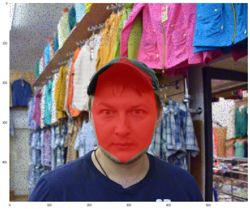

Fuzzy separation of background and object

Now we have two data sets: object points $D_f$ and background points $D_b$ .

 points_fg = np.array([img_input[x, y, :] for (x, y) in xy_fg]) points_bg = np.array([img_input[x, y, :] for (x, y) in xy_bg])

Let's look at the distribution of colors on the RGB channels in each of the sets. The first histogram is for the object, the second is for the background.

drawing distributions

 fig, axes = plt.subplots(nrows=2, ncols=1) sns.distplot(points_fg[:, 0], ax=axes[0], color='r') sns.distplot(points_fg[:, 1], ax=axes[0], color='g') sns.distplot(points_fg[:, 2], ax=axes[0], color='b') sns.distplot(points_bg[:, 0], ax=axes[1], color='r') sns.distplot(points_bg[:, 1], ax=axes[1], color='g') sns.distplot(points_bg[:, 2], ax=axes[1], color='b')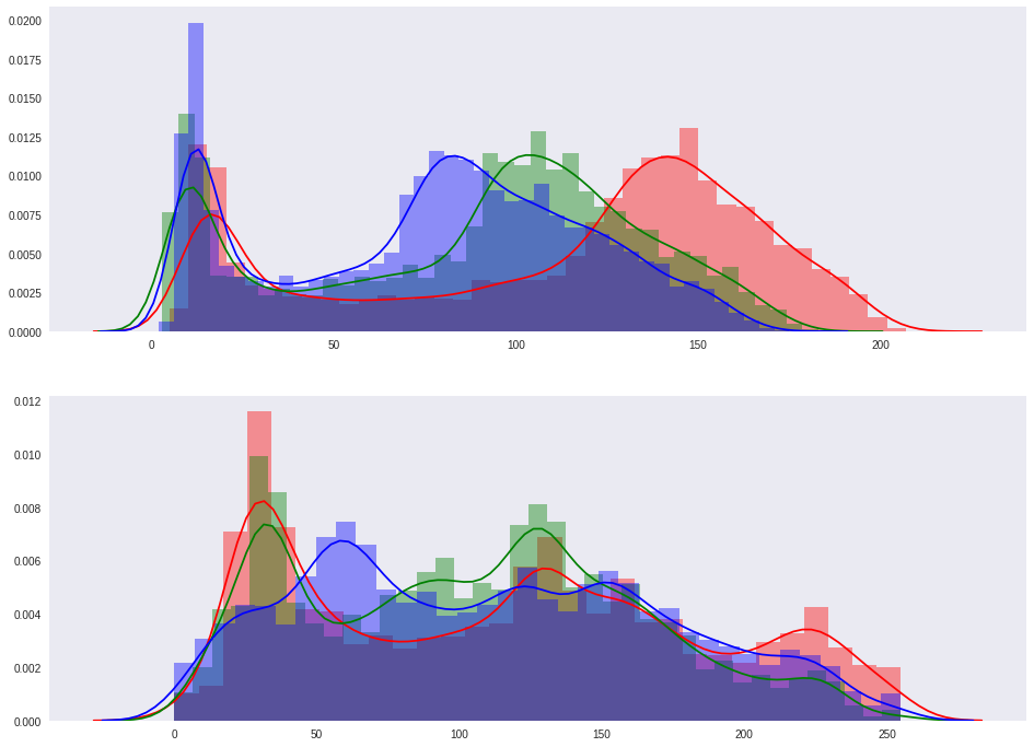

I am glad that the distributions are different. This means that if we can get functions that estimate the probability that a point belongs to the desired distribution, then we will get fuzzy masks. And there is such a way - kernel density estimation . For a given set of points, you can build a density estimate function for a new point. $x$ as follows (for simplicity, an example for a one-dimensional distribution):

F l e f t (x r i g h t) = f r a c 1 h c d o t l e f t | D r i g h t | s u m_{i = 1}^{l e f t | D r i g h t |} K l e f t (f r a c x - x_{i} h r i g h t)

$F \ left (x \ right) = \ frac {1} {h \ cdot \ left | D \ right |} \ sum_ {i = 1} ^ {\ left | D \ right |} K \ left (\ frac {x - x_i} {h} \ right)$

Where:

$h$ - smoothing parameter
$K$ - some core

For simplicity, we will use the Gaussian core:

K (u) = f r a c 1 s q r t 2 p i e^{- f r a c 12 u^{2}}

$K (u) = {\ frac {1} {\ sqrt {2 \ pi}}} e ^ {- {\ frac {1} {2}} u ^ {2}}$

Although the speed of the Gaussian core is not the best choice, and if you take the Eepanechnikov core , then everything will be considered faster. I will also use KerleDensity from sklearn , which will eventually result in 5 minutes of scoring. The authors of this article argue that replacing KDE with an optimal implementation reduces the calculations on the device to one second.

 #   KDE     kde_fg = KernelDensity(kernel='gaussian', bandwidth=1, algorithm='kd_tree', leaf_size=100).fit(points_fg) kde_bg = KernelDensity(kernel='gaussian', bandwidth=1, algorithm='kd_tree', leaf_size=100).fit(points_bg) #     score_kde_fg = np.zeros(img_input.shape[:2]) score_kde_bg = np.zeros(img_input.shape[:2]) likelihood_fg = np.zeros(img_input.shape[:2]) coodinates = it.product(range(score_kde_fg.shape[0]), range(score_kde_fg.shape[1])) for x, y in tqdm_notebook(coodinates, total=np.prod(score_kde_fg.shape)): score_kde_fg[x, y] = np.exp(kde_fg.score(img_input[x, y, :].reshape(1, -1))) score_kde_bg[x, y] = np.exp(kde_bg.score(img_input[x, y, :].reshape(1, -1))) n = score_kde_fg[x, y] + score_kde_bg[x, y] if n == 0: n = 1 likelihood_fg[x, y] = score_kde_fg[x, y]/n

As a result, we have several masks:

score_kde_fg - estimation of the probability of being a point of an object $p \ left (x \ mid D_f \ right)$
score_kde_bg - estimation of the probability of being a point of the background $p \ left (x \ mid D_b \ right)$
likelihood_fg - normalized probability of being a point on an object $p_f \ left (x \ right) = \ frac {p \ left (x \ mid D_f \ right)} {p \ left (x \ mid D_f \ right) + p \ left (x \ mid D_b \ right)}$
1 - likelihood_fg normalized probability of being a background point $p_b \ left (x \ right) = 1 - p_f \ left (x \ right)$

Look at the following distributions.

The distribution of score_kde_fg values

 sns.distplot(score_kde_fg.flatten()) plt.show()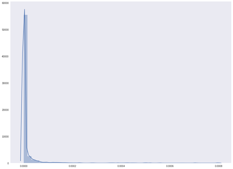

The distribution of score_kde_bg

 sns.distplot(score_kde_bg.flatten()) plt.show()

The distribution of values likelihood_fg:

 sns.distplot(likelihood_fg.flatten()) plt.show()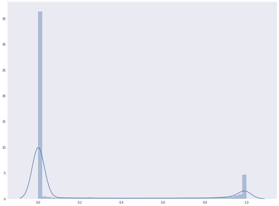

Instilling hope that $p_f \ left (x \ right)$ there are two peaks, and the number of points belonging to the face is clearly not less than the background points. Draw the resulting mask.

mask score_kde_fg

 plt.matshow(score_kde_fg, cmap=cm.bwr) plt.show()

mask score_kde_bg

 plt.matshow(score_kde_bg, cmap=cm.bwr) plt.show()

 plt.matshow(likelihood_fg, cmap=cm.bwr) plt.show()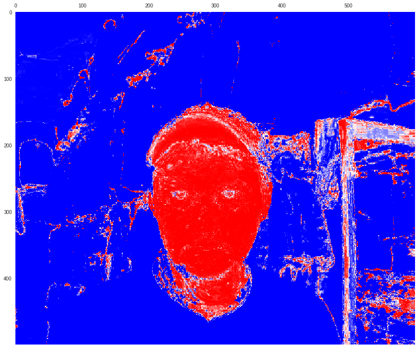

mask 1 - likelihood_fg

 plt.matshow(1 - likelihood_fg, cmap=cm.bwr) plt.show()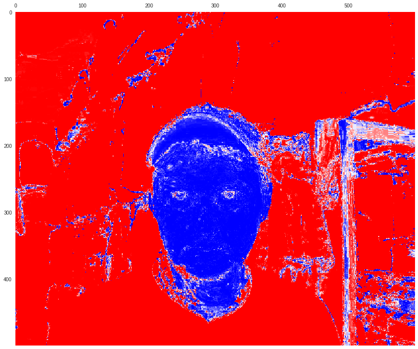

Unfortunately, part of the door jamb turned out to be part of the face. Well, that cant far from the face. We will use this property in the next part.

Binary object mask

Imagine the image as a graph, the nodes of which are pixels, and the edges are connected to the points above and below the current point, as well as to the right and left of it. The weights of the edges will be the absolute value of the difference in the probabilities of belonging points to an object or to the background:

d l e f t (a, b r i g h t) = l e f t | p l e f t (a r i g h t) - p l e f t (b r i g h t) r i g h t |

$d \ left (a, b \ right) = \ left | p \ left (a \ right) - p \ left (b \ right) \ right |$

Accordingly, the closer the probabilities are to each other, the lower is the edge weight between points. We use the Dijkstra algorithm to find the shortest paths and their distances from the point to all the others. We will call the algorithm two times, applying to the input all the probabilities of belonging in the object and then the probabilities of belonging of points to the background. The concept of distance is sewn directly into the algorithm, and the distance between points belonging to one group (object or background) will be zero. As part of the Dijkstra algorithm, we can put all these points in the group of visited vertices.

 def dijkstra(start_points, w): d = np.zeros(w.shape) + np.infty v = np.zeros(w.shape, dtype=np.bool) q = queue.PriorityQueue() for x, y in start_points: d[x, y] = 0 q.put((d[x, y], (x, y))) for x, y in it.product(range(w.shape[0]), range(w.shape[1])): if np.isinf(d[x, y]): q.put((d[x, y], (x, y))) while not q.empty(): _, p = q.get() if v[p]: continue neighbourhood = [] if p[0] - 1 >= 0: neighbourhood.append((p[0] - 1, p[1])) if p[0] + 1 <= w.shape[0] - 1: neighbourhood.append((p[0] + 1, p[1])) if p[1] - 1 >= 0: neighbourhood.append((p[0], p[1] - 1)) if p[1] + 1 < w.shape[1]: neighbourhood.append((p[0], p[1] + 1)) for x, y in neighbourhood: #    d_tmp = d[p] + np.abs(w[x, y] - w[p]) if d[x, y] > d_tmp: d[x, y] = d_tmp q.put((d[x, y], (x, y))) v[p] = True return d #      d_fg = dijkstra(xy_fg, likelihood_fg) d_bg = dijkstra(xy_bg, 1 - likelihood_fg)

new fuzzy object mask

 plt.matshow(d_fg, cmap=cm.bwr) plt.show()

new fuzzy background mask

 plt.matshow(d_bg, cmap=cm.bwr) plt.show()

And now we refer to the object all those points from which the distance to the object is less than the distance to the background (you can add a gap).

 margin = 0.0 mask = (d_fg < (d_bg + margin)).astype(np.uint8) plt.matshow(mask) plt.show()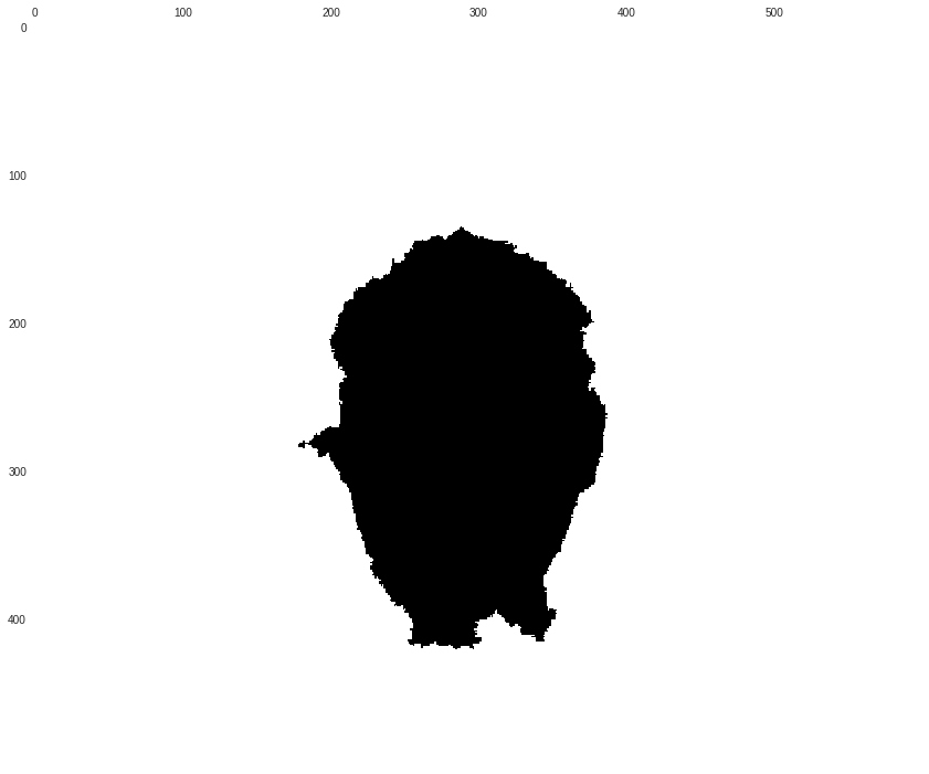

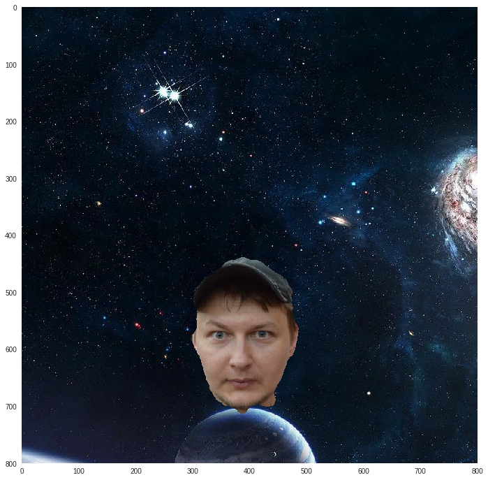
You can send yourself into space.

 img_fg = img_input/255.0 img_bg = (np.array(Image.open('./../data/background.jpg'))/255.0)[:800, :800, :] x = int(img_bg.shape[0] - img_fg.shape[0]) y = int(img_bg.shape[1]/2 - img_fg.shape[1]/2) img_bg_fg = img_bg[x:(x + img_fg.shape[0]), y:(y + img_fg.shape[1]), :] mask_3d = np.dstack([mask, mask, mask]) img_bg[x:(x + img_fg.shape[0]), y:(y + img_fg.shape[1]), :] = mask_3d*img_fg + (1 - mask_3d)*img_bg_fg plt.imshow(img_bg)

Mask smoothing

You probably noticed that the mask is slightly torn at the edges. But this is easily corrected by the methods of mathematical morphology .

Suppose we have a structural element (FE) of the type "disk" - a binary disk mask.

erosion: we apply to each point of the object on the original image of the FE so that the center of the FE and the point on the image coincide; if the FE completely belongs in the object, then such a point of the object remains; it turns out that parts that are smaller than the ESS are removed, and the object "loses weight"; in the example of the blue square made blue
dilation: an EF is superimposed on each point of the object, and the missing points are drawn; thus, holes smaller than the solar cell are painted over, and the object as a whole "gets fatter"; the example of a blue square made blue, the corners turned out rounded
opening (opening): first erosion, then build-up with the same EF
closing (closing): first building up, then erosion with the same AU

We will use the opening, which will first remove the "hairiness" at the edges, and then return the original size (the object will "lose weight" after erosion).

 mask = morphology.opening(mask, morphology.disk(11)) plt.imshow(mask)

After applying such a mask, the result will be more pleasant:

mask application code

 img_fg = img_input/255.0 img_bg = (np.array(Image.open('./../data/background.jpg'))/255.0)[:800, :800, :] x = int(img_bg.shape[0] - img_fg.shape[0]) y = int(img_bg.shape[1]/2 - img_fg.shape[1]/2) img_bg_fg = img_bg[x:(x + img_fg.shape[0]), y:(y + img_fg.shape[1]), :] mask_3d = np.dstack([mask, mask, mask]) img_bg[x:(x + img_fg.shape[0]), y:(y + img_fg.shape[1]), :] = \ mask_3d*img_fg + (1 - mask_3d)*img_bg_fg plt.imshow(img_bg)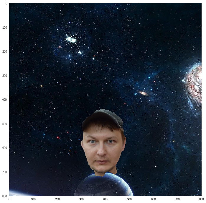

Mask down

Take a random picture from the Internet for the face transfer experiment.

Test copy

 img_target = np.array(Image.open('./../data/target.jpg')) img_target = (transform.rescale(img_target, scale=0.5, mode='constant')*255).astype(np.uint8) print(img_target.shape) plt.imshow(img_target)

We find on the experimental all 68 prickly points of the face, I remind you that they will be in the same order as on any other face.

 img_gray = cv2.cvtColor(img_target, cv2.COLOR_BGR2GRAY) rects_target = detector(img_gray, 0) shape_target = predictor(img_gray, rects_target[0]) shape_target = face_utils.shape_to_np(shape_target)

To transfer one person to another, you need to scale the first person under a new one, rotate it and move it, i.e. apply some affine transformation to the first person. It turns out that the affine transformation is not some, but quite specific. It should be such that translates 68 points of the first person to 68 points of the second person. It turns out that to obtain an affine transform operator, we need to solve the linear regression problem.

l e f t (b e g i n a r r a y c c x_{1}^{1}, x_{1}^{2}, 1 x_{2}^{1}, x_{2}^{2}, 1 c d o t s x_{68}^{1}, x_{68}^{2}, 1 e n d a r r a y r i g h t) t i m e s l e f t (b e g i n a r r a y c c a_{1}^{1}, a_{2}^{1}, a_{3}^{1} a_{1}^{2}, a_{2}^{2}, a_{3}^{2} a_{1}^{3}, a_{2}^{3}, a_{3}^{3} e n d a r r a y r i g h t) = l e f t (b e g i n a r r a y c c y_{1}^{1}, y_{1}^{2}, 1 y_{2}^{1}, y_{2}^{2}, 1 c d o t s y_{68}^{1}, y_{68}^{2}, 1 e n d a r r a y r i g h t)

$\ left (\ begin {array} {cc} x ^ 1_1, x ^ 2_1, 1 \\ x ^ 1_2, x ^ 2_2, 1 \\ \ cdots \\ x ^ 1_ {68}, x ^ 2_ {68 }, 1 \ end {array} \ right) \ times \ left ({\ begin {array} {cc} a_1 ^ 1, a_2 ^ 1, a_3 ^ 1 \\ a_1 ^ 2, a_2 ^ 2, a_3 ^ 2 \ \ a_1 ^ 3, a_2 ^ 3, a_3 ^ 3 \\ \ end {array}} \ right) = \ left ({\ begin {array} {cc} y ^ 1_1, y ^ 2_1, 1 \\ y ^ 1_2 , y ^ 2_2, 1 \\ \ cdots \\ y ^ 1_ {68}, y ^ 2_ {68}, 1 \ end {array}} \ right)$

This equation is easily solved using a pseudoinverse matrix :

l a r g e X c d o t A = Y R i g h t a r r o w A = l e f t (X^{T} X r i g h t)^{- 1} X^{T} Y

$\ large X \ cdot A = Y \ Rightarrow A = \ left (X ^ T X \ right) ^ {- 1} X ^ T Y$

So do:

 #      , #      ,   X = np.hstack((shape, np.ones(shape.shape[0])[:, np.newaxis])) Y = np.hstack((shape_target, np.ones(shape_target.shape[0])[:, np.newaxis])) #   A = np.dot(np.dot(np.linalg.inv(np.dot(XT, X)), XT), Y) #       X = np.array([(y, x, 1) for (x, y) in it.product(range(mask.shape[0]), range(mask.shape[1])) if mask[x, y] == 1.0]) #        Y = np.dot(X, A).astype(np.int)

Mask down

 img_tmp = img_target.copy() for y, x, _ in Y: if x < 0 or x >= img_target.shape[0] or y < 0 or y >= img_target.shape[1]: continue img_tmp[x, y, :] = np.array([0, 0, 0]) plt.imshow(img_tmp)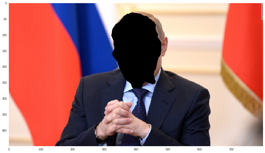

Transfer face

 img_trans = img_target.copy().astype(np.uint8) points_face = {} for ix in range(X.shape[0]): y1, x1, _ = X[ix, :] y2, x2, _ = Y[ix, :] if x2 < 0 or x2 >= img_target.shape[0] or y2 < 0 or y2 >= img_target.shape[1]: continue points_face[(x2, y2)] = img_input[x1, y1, :] for (x, y), c in points_face.items(): img_trans[x, y, :] = c plt.imshow(img_trans)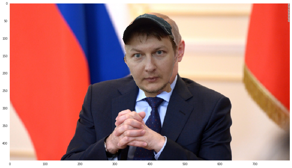

Conclusion

As homework, you can make the following improvements yourself:

add transparency around the edges, so that a smooth transition of the mask to the target image (matting);
Fix the transfer to larger images - the points of the original face are not enough to cover all the points of the target face, thus, gaps between the points are formed; This can be corrected by increasing the size of the original face;
make some kind of mask, such as Dale Chipmunk , manually apply 68 points and carry out the transfer (here's a masquerade);
use some trendy neural network point detector that can search for more points.

The source notebook is here . Have a great time.

As usual ATP bauchgefuehl for editing.

Source: https://habr.com/ru/post/336594/

All Articles