I love stories about the apocalypse, about how our planet is enslaved by aliens, monkeys or terminators, and from childhood I dreamed of bringing the last day of humanity closer.

However, I do not know how to build flying saucers or synthesize viruses, and therefore it will be a question of terminators, or rather, how to help these laborers to find John Connor.

My handmade terminator will be somewhat simplified - he will not be able to walk, shoot, say "I'll be back". The only thing he will be able to do is recognize Connor’s voice if he hears him (or, for example, Churchill, if he also has to be found).

General scheme

Any recognition system works in two modes: in the registration mode and the identification mode. In other words, you need to have an example voice.

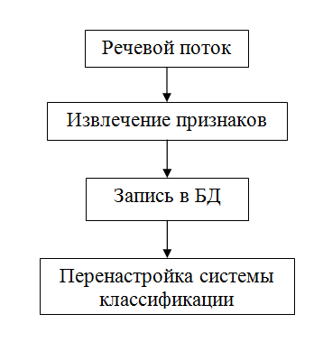
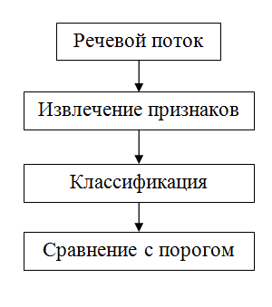
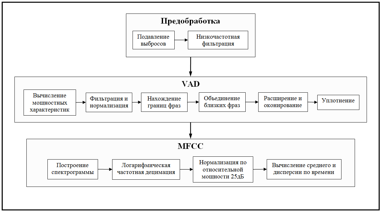
The pictures above show the general scheme of the system in each of the modes. As you can see, these modes are very similar. Both of them need to capture the speech audio stream and calculate its main features. The difference is what to do with these signs. When registering them, one way or another you need to somehow remember for future use. It is much more efficient to work with the main features than with the original raw data. When identifying, nothing can be saved, since the system at this stage has no feedback and cannot reliably know the belonging of the voice.

Classifiers

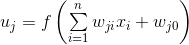
What are the "signs"? In fact, this is just a set of numbers characterizing the speaker - a vector in multidimensional space. And the task of the classifier is to build a function mapping this multidimensional space into the space of real numbers. In other words, his task is to obtain a number that would characterize the measure of similarity.

• Euclid $$$\ qquad \ qquad D = \ sqrt {\ sum \ limits_ {i = 1} {\ left | {x_i} \ right |}} \ qquad \ qquad \ qquad$Euclidean distance
• SVM $$$\ qquad \ qquad y = \ left \ langle {\ mathbf {w, x}} \ right \ rangle + w_0 \ qquad \ qquad \ quad \;$Split hyperplane
• MLP $$$\ qquad \ qquad$$$$\ qquad$ Network of nonlinear functions

Experiments

Binary classification

For the binary classification, the task of recognizing the gender of the speaker was chosen. Thus, there are only 3 clearly defined possible outcomes: male voice, female voice, unknown.

Two series of experiments were carried out. In the first case, the test was carried out on the same data on which the system was configured. In the second case, testing was conducted on audio recordings of people whose data the system does not have, and the ability of the method to generalize was tested.

Euclid

In this case, the average value of the vectors of signs for the male and female votes was calculated, after which the Euclidean distance of the tested voice was found with each of the average, on the result of which the choice was made.

To calculate the threshold value, the average value of the distance inside the group and between the groups was found, after which normalization to one occurred.

A positive value relative to the threshold is the classification of the female voice. Negative - male.

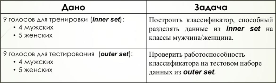
SVM

For this method, an array containing a binary value was created, the positive value of which corresponded to the female voice. This binary array together with the matrix of training signs was fed to the input of the algorithm, after which the testing took place.

In this case, the threshold is the number 0, since all positive results must correspond to one class, negative - to another. However, to improve comparison with other methods, the results were compressed by 2 times and shifted by 0.5.

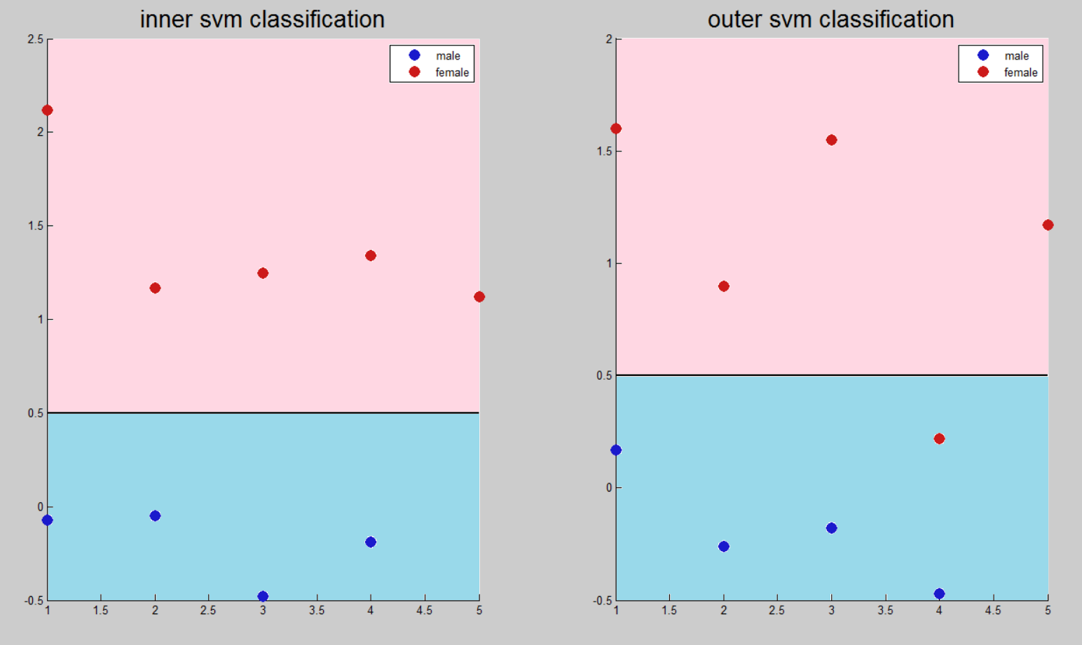
MLP

The task of multilayer perceptron is to approximate functions, and not binary classification. In this regard, there is no separating threshold, but there is an interval near the ideal value in which the neural network gives the result.

When setting the vectors of signs of female voices, the value 1 was set in correspondence, for men - 0.

Authentication task

To test the possibility of generalizing the algorithm, an additional test was performed on a set that did not correspond to the initial one.

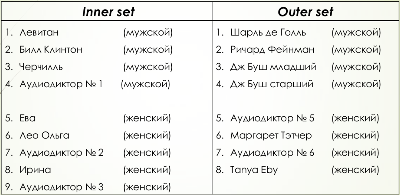
In the source table there are 9 columns and 9 rows, since the check was carried out on the principle of each with each, and only 9 samples of people in the initial set. In the generalized table, there are 9 columns and 8 rows, since there are only 8 people in the test set that differ from the initial set

Euclid

Classification by "learnable" set. Although for this algorithm, the concept of "learnable set" is not applicable, since the learning itself does not occur. The average values ​​of the distances inside the class and between the classes and the normalization are calculated: the value of 1 is assigned to the first case, otherwise - 0.

As a result, the authentication matrix should ideally contain units on the main diagonal and zeros in all other cells.

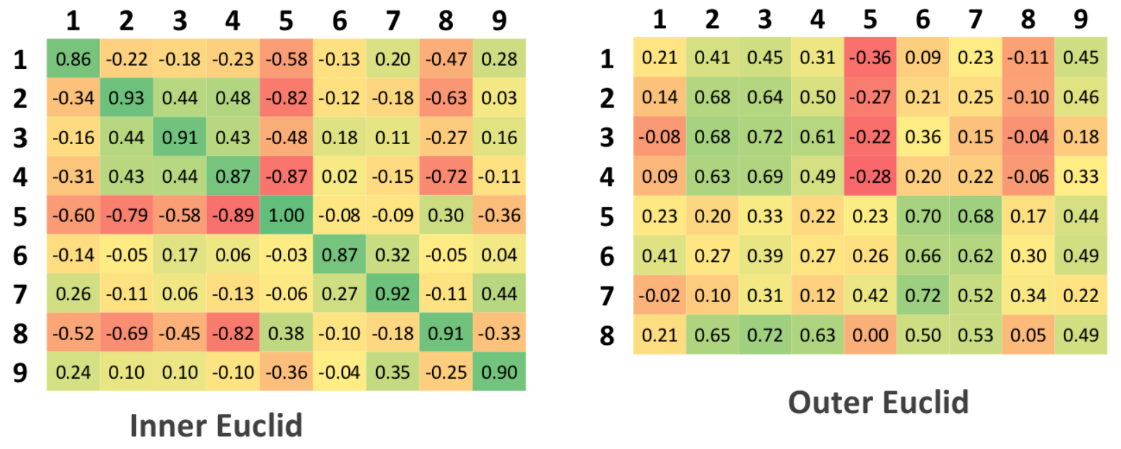
For the matrix under test, ideally, there should be no more values ​​than those that stood on the main diagonal of the authentication matrix, which corresponds to the fact that the algorithm was able to detect a discrepancy between the source and test data

SVM

Since the support vector machines solve the problem of binary, rather than multi-class classification, 9 different SVMs were created for the authentication task, each of which is configured for a specific person, and the others are considered as negative
example of classification.

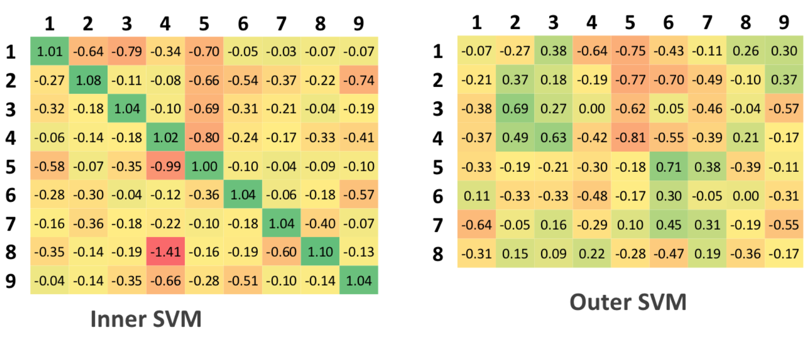
The interpretation of table data for SVM is similar to the tables for the Euclidean algorithm, i.e. 0.5 is a threshold value.

MLP

To use a multilayer perceptron, at the configuration stage, 9-dimensional vectors were fed as output values ​​of the system. In this case, for each input feature vector at the output of the MLP, approximated the values ​​of 9 functions responsible for the classification task.

As in the case of a binary classification, there is no threshold value that would unambiguously classify the class of the input vector, but there is some interval around ideal values. Any way out of the interval indicates the inability of the network with a given level of confidence interval to give a clear answer.

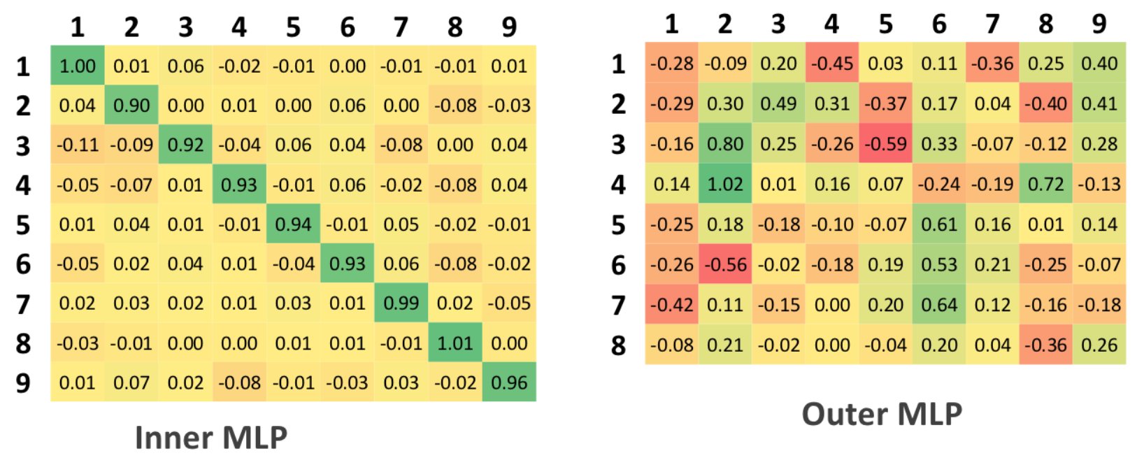
Additionally, it should be noted that the confidence interval cannot be greater than 0.5, since this value is equal to half the value between the ideal classification values.

Comparison of classification methods

The most notable results obtained during the experiments are the low level of accuracy by the Euclidean method and the very high computational costs of setting up a multilayer perceptron: the duration of the MLP setup exceeded the duration of the SVM setup several hundred times on the same data set.

The results of the binary classification suggest that all three methods coped well with the entire test set, except for the voice of Tanya Eby, which was mistakenly classified by all methods. This result can be explained by the rudeness of the woman’s voice.

The solution of the problem of multi-class classification for neural network systems, as it turned out, is strikingly different for cases of “internal” and “external” authentication. If in the first case both neural network methods coped with the task, in the second case both made a number of erroneous classifications.

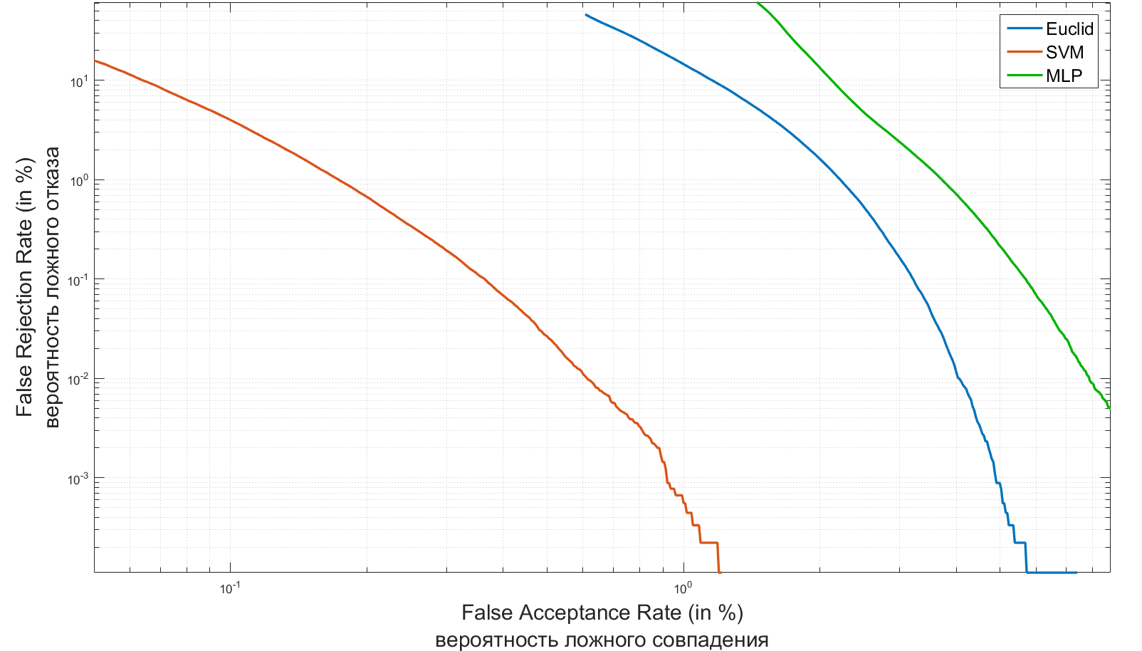
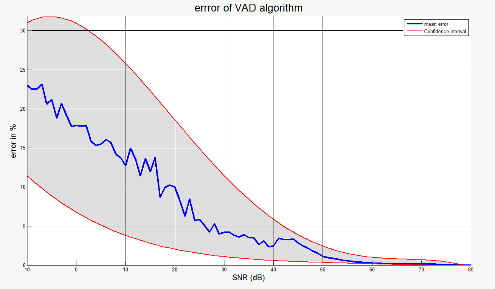
As the two main characteristics of any identification system, errors of the first and second kind can be accepted. In the theory of radar, they are usually called “false alarm” or “target omission”, and in identification systems, the most well-established concepts are FAR (False Acceptance Rate) and FRR (False Rejection Rate). The first number describes the probability of a false coincidence of the biometric characteristics of two people. The second is the probability of denial of access to a person who has access. The system is the better, the lower the FRR value for the same FAR values.

Below are the FAR / FRR graphics of the systems I created for the authentication task.

A good overview of biometric identification systems and an assessment of their FAR / FRR values ​​can be found here .

Euclid :

• The fastest and easiest algorithm
• Scaling performance degradation
• Low quality classification

SVM :

• The best generalizing ability
• Requires small computing resources at the training stage
• The need to create N different SVM

MLP :

• The smallest learning error
• No classification concept
• Demanding computing resources at the training stage
• The need to retrain the entire system when registering a new speaker

Sound traps

All audio information is received by the system as an array of audio stream and quantization frequency values.

An array is formed by reading from files mp3, flac, wav or any other format, the necessary fragment is cut, averaged into one track and the constant component is subtracted:

filename = 'sample/Irina.mp3'; [x, fs] = audioread(filename); % x -  - % fs -   %%   sec_start = 0.5; sec_stop = 10; frame_start = max(sec_start*fs, 1); frame_stop = min(length(x), sec_stop*fs); sec_start = (frame_start / fs) - fs; sec_stop = frame_stop / fs; %%  x = x(frame_start : frame_stop, :); x = mean(x, 2); x = x - mean(x); 

Feature extraction

Pretreatment

Even though our terminator is budgetary, even it cannot do without digital processing. The task of pre-filtering was to get rid of the noise characteristics of audio recordings that most affect the algorithm for further processing. Such characteristics were chosen "emissions" and "low frequency" noise.

Emissions

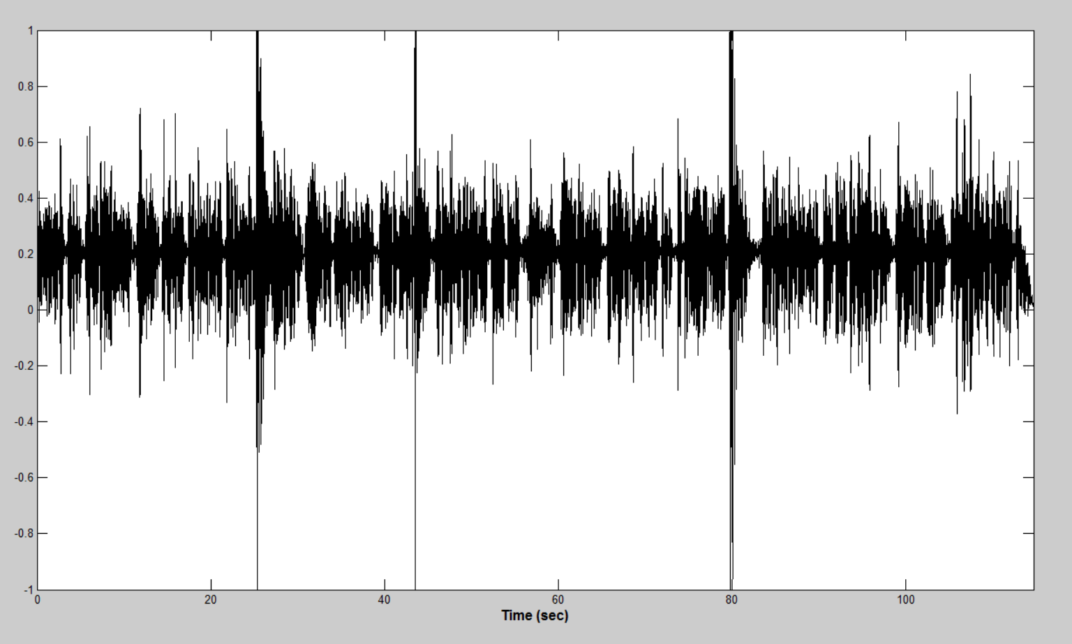
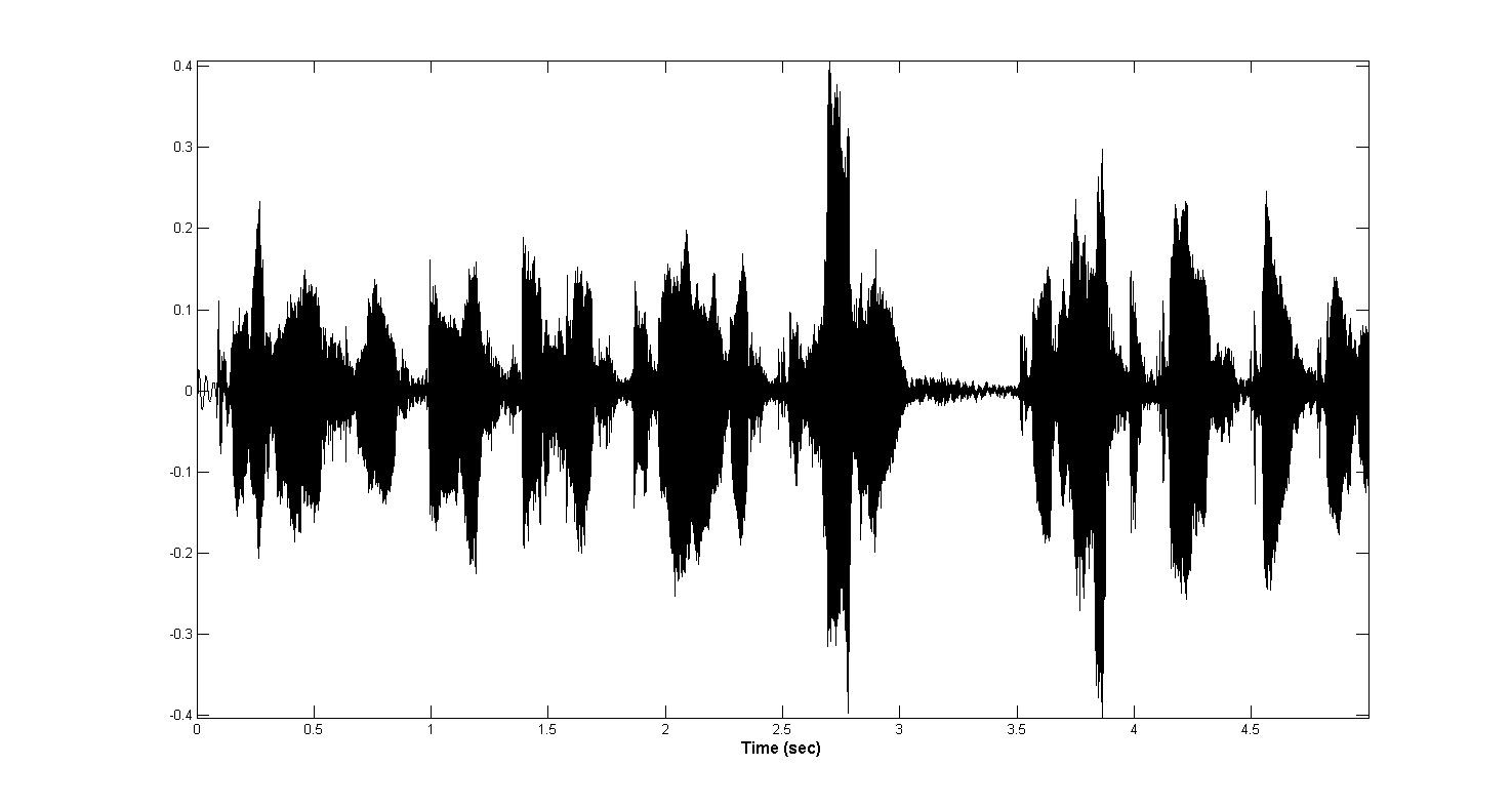
The microphones with which I recorded voices turned out to be quite different in quality. Poor sound recording equipment led to short-term power surges. These noise phenomena can provide great difficulties for the algorithm for finding voice activity. An example of such “emissions” is shown in the figure below.

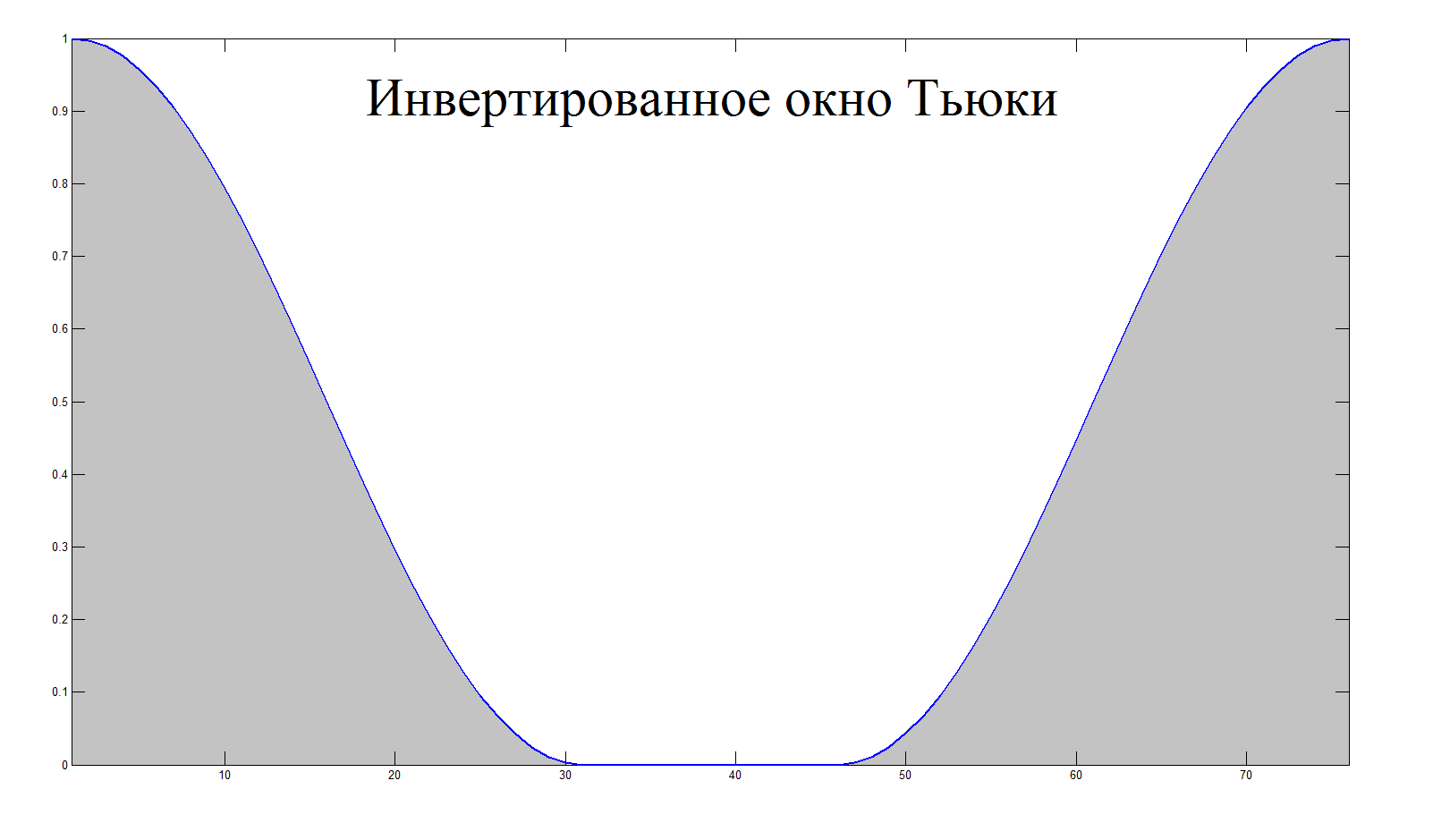
The idea of ​​the algorithm is to sequentially calculate the energy of short sections, comparing with the average energy value and suppressing by multiplying with the Tukey's inverted window in case of exceeding the energy of the segment of the average value by
some threshold. For smoother filtering and accurate detection, the intermediate sections of the audio file were selected with overlapping.

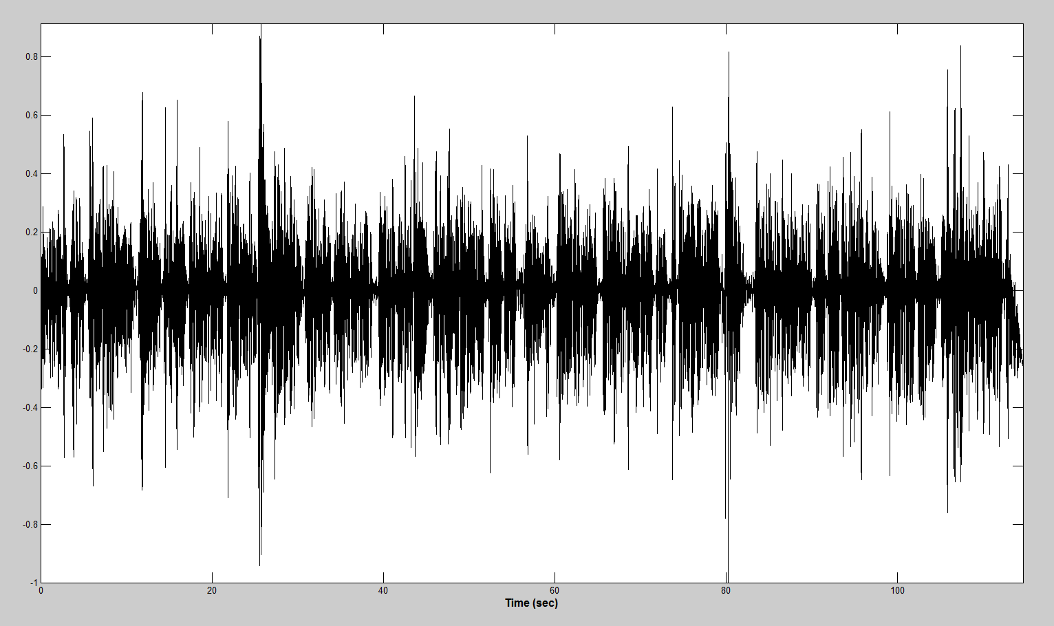
 function [ y ] = outlier_suppression( x, fs ) buffer_duration = 0.1; % in seconds accumulation_time = 3; % in seconds overlap = 50; % in percent outlier_threshold = 7; buffer_size = round( ((1 + 2*(overlap / 100))*buffer_duration) * fs); sample_size = round(buffer_duration * fs); y = x; cumm_power = 0; amount_iteration = floor(length(y) / sample_size); for iter = 1 : amount_iteration start_index = (iter - 1) * sample_size; start_index = max(round(start_index - (overlap / 100)*sample_size), 1); end_index = min(start_index + buffer_size, length(x)); buffer = y(start_index : end_index); power = norm(buffer); if ((accumulation_time/buffer_duration < iter) && ((outlier_threshold*cumm_power/iter) < power)) buffer = buffer .* (1 - tukeywin(end_index - start_index + 1, 0.8)); y(start_index : end_index) = buffer; cumm_power = cumm_power + (cumm_power/iter); continue end cumm_power = cumm_power + power; end end 

After processing, the sample presented above looks like this:

Low frequency noise

Low frequency harmonics are dangerous in that they create a constant energy component in a short period of time, which can be erroneously recognized as voice activity if the necessary measures are not taken.

To get rid of such components, an elliptical third-order high - pass filter with a cut-off frequency of 30 Hz was selected, and providing 20 dB suppression in the stopband. The choice of elliptical filter was made due to the fact that elliptical filters provide a steeper (compared to Butterworth and Chebyshev filters) decrease in the frequency response in the transition zone between the passbands and the delay band. The price for this is the presence of uniform pulsation of the frequency response in both the passband and the stopband.

Below are the signals before and after filtering, respectively:

Voice Activity Detection

The system for allocating time segments of voice activity built by me is based exclusively on the power characteristics of the signal and noise. In some ways, this was a compromise between a simple calculation of the norm and a complex processing of the spectra of the time matrix. The bonus was a sharp decrease in the dimension of the arrays (several thousand times), which turned out to be very helpful, given the intensity of access to the data.

Calculation of power characteristics

The following formulas were used as the power characteristics of the signal and noise: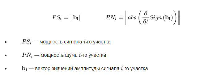

 function [ signal_power_array, noise_power_array ] = compute_power_arrays(x,fs) buffer_duration = 10 * 10^(-3); % in seconds overlap = 50; % in percent sample_size = round(buffer_duration * fs); buffer_size = round( ((1 + 2*(overlap / 100))*buffer_duration) * fs); signal_power_array = zeros(floor(length(x) / sample_size), 1); noise_power_array = zeros(length(signal_power_array), 1); for iter = 1 : length(signal_power_array) start_index = (iter - 1) * sample_size; start_index = max(round(start_index - (overlap / 100)*sample_size), 1); end_index = min(start_index + buffer_size, length(x)); buffer = x(start_index : end_index); signal_power_array(iter) = norm(buffer); noise_power_array(iter) = norm(abs(diff(sign(buffer)))); end end 

 %% filtering gw = gausswin(8); signal_power_array = filter(gw, 1, signal_power_array); signal_power_array = signal_power_array - base_value(signal_power_array); signal_power_array = max(signal_power_array, 0); signal_power_array = signal_power_array ./ max(signal_power_array); gw = gausswin(16); noise_power_array = filter(gw, 1, noise_power_array); noise_power_array = noise_power_array - base_value(noise_power_array); noise_power_array = max(noise_power_array, 0); noise_power_array = -noise_power_array + max(noise_power_array); noise_power_array = noise_power_array ./ max(noise_power_array); noise_power_array = (1 - noise_power_array); 

 function [ value ] = base_value( array ) [nelem, centres] = hist(array, 100); [~, index_max] = max(nelem); value = centres(index_max); end 

Finding the boundaries of phrases

To find the boundaries of the phrases, the signal power array is passed in both directions. In each case, the decay of energy is sought, and since the array is traversed in two directions, both the beginning and the end of the phrases are found.

 %% find the end of phrases phrase_detection = zeros(size(signal_power_array)); max_magn = 0; for iter = 1 : length(signal_power_array) max_magn = max(max_magn, signal_power_array(iter)); if (signal_power_array(iter) < 2*threshold*max_magn) phrase_detection(iter) = 1; max_magn = 0; end end %% find the start of phrases max_magn = 0; for iter = length(signal_power_array) : -1 : 1 max_magn = max(max_magn, signal_power_array(iter)); if (signal_power_array(iter) < 2*threshold*max_magn) phrase_detection(iter) = 1; max_magn = 0; end end %% post processing of phrase detection array phrase_detection = not(phrase_detection); phrase_detection(1) = 0; phrase_detection(end) = 0; edge_phrase = diff(phrase_detection); %% create phrase array phrase_counter = 0; for iter = 1 : length(edge_phrase) if (0 < edge_phrase(iter)) phrase_counter = phrase_counter + 1; phrase(phrase_counter).start = iter; elseif (edge_phrase(iter) < 0) start = phrase(phrase_counter).start; phrase(phrase_counter).end = iter; phrase(phrase_counter).power = mean(signal_power_array(start : iter)); phrase(phrase_counter).noise_power = mean(noise_power_array(start : iter)); end end 

Combining phrases

Often the duration of the calculated phrases is less than 100ms. In this regard, an algorithm has been developed that combines short closely spaced phrases into one. For this, the energies of the neighboring areas are compared, and if they differ by less than the set threshold, these areas are combined. At the same time, the energy of the combined phrases was recalculated in proportion to the duration and power of each.

 %% union small phrases length_threshold = 16; iter = 1; while (iter < length(phrase)) phrase_length = phrase(iter).end - phrase(iter).start; if ((phrase_length<length_threshold) && (iter<length(phrase)) && (iter~=1)) lookup_power = phrase(iter+1).power; behind_power = phrase(iter-1).power; if (abs(lookup_power-phrase(iter).power) < abs(behind_power-phrase(iter).power)) next_iter = iter + 1; else next_iter = iter - 1; end power_ratio = phrase(next_iter).power / phrase(iter).power; power_ratio = min(power_ratio, 1 / power_ratio); if ( power_ratio < threshold ) iter = iter + 1; continue; end min_index = min(phrase(iter).start, phrase(next_iter).start); max_index = max(phrase(iter).end, phrase(next_iter).end); phrase_next_length = (phrase(next_iter).end - phrase(next_iter).start); phrase(next_iter).power = ... ((phrase(iter).power*phrase_length)+(phrase(next_iter).power*phrase_next_length)) / (phrase_length + phrase_next_length); phrase(next_iter).noise_power = ... ((phrase(iter).noise_power*phrase_length)+phrase(next_iter).noise_power*phrase_next_length)) / (phrase_length + phrase_next_length); phrase_detection((min_index+1) : (max_index-1)) = phrase_detection(phrase(next_iter).start+1); phrase(next_iter).start = min_index; phrase(next_iter).end = max_index; phrase(iter) = []; else iter = iter + 1; end end 

 %% union neibours phrases threshold = 0.1; iter = 1; while (iter <= length(phrase)) if (phrase_power_threshold < phrase(iter).power) phrase(iter).voice = 1; elseif ((phrase_power_threshold < 5*phrase(iter).power) ... && (phrase(iter).noise_power < 0.5*phrase(iter).power)) phrase(iter).voice = 1; else phrase(iter).voice = 0; end if (iter ~= 1) if (phrase(iter-1).voice == phrase(iter).voice) phrase(iter-1).end = phrase(iter).end; phrase_detection(phrase(iter-1).start+1 : phrase(iter-1).end-1) = phrase(iter-1).voice; phrase(iter) = []; continue; end end iter = iter + 1; end 

For a smooth transition between periods of activity and lull, the arrays of phrases are extended by 50ms in each direction (if possible). Before this, in order to map the indices to time intervals, the indices of the power arrays are recalculated into the indices of the audio stream.

 %% compute real sample indexes for iter = 1 : length(phrase) start_index = (phrase(iter).start - 1) * sample_size + 1; end_index = phrase(iter).end * sample_size; phrase(iter).start = start_index; phrase(iter).end = end_index; end phrase(1).start = 1; phrase(end).end = length(x); %% spread voice in time spread_voice = round(50 * 10^(-3) * fs); iter = 2; while (iter < length(phrase)) if (phrase(iter).voice) phrase(iter).start = phrase(iter).start - spread_voice; phrase(iter).end = phrase(iter).end + spread_voice; else phrase(iter).start = phrase(iter - 1).end + 1; phrase(iter).end = phrase(iter + 1).start - 1 - spread_voice; end phrase(iter).start = max(phrase(iter).start, 1); phrase(iter).end = min(phrase(iter).end, length(x)); if (phrase(iter).start < phrase(iter).end) iter = iter + 1; else phrase(iter-1).end = phrase(iter).end; phrase(iter) = []; end end phrase(1).start = 1; phrase(1).end = phrase(2).start - 1; phrase(end).start = phrase(end - 1).end + 1; phrase(end).end = length(x); 

After all the voice activity sections have been found and the initial and final indices of each of the phrases have been calculated, an array is created that will contain the full audio signal of the activity sections. These areas are multiplied by the Kaiser window function to reduce spreading of the spectrum. The Kaiser window is selected due to the small inflection values.

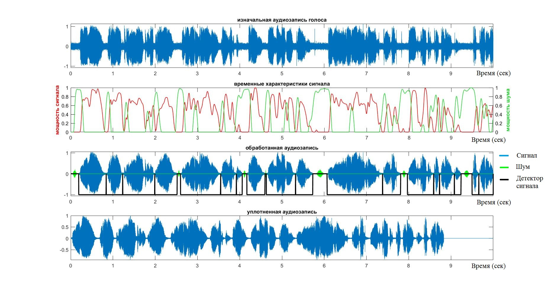
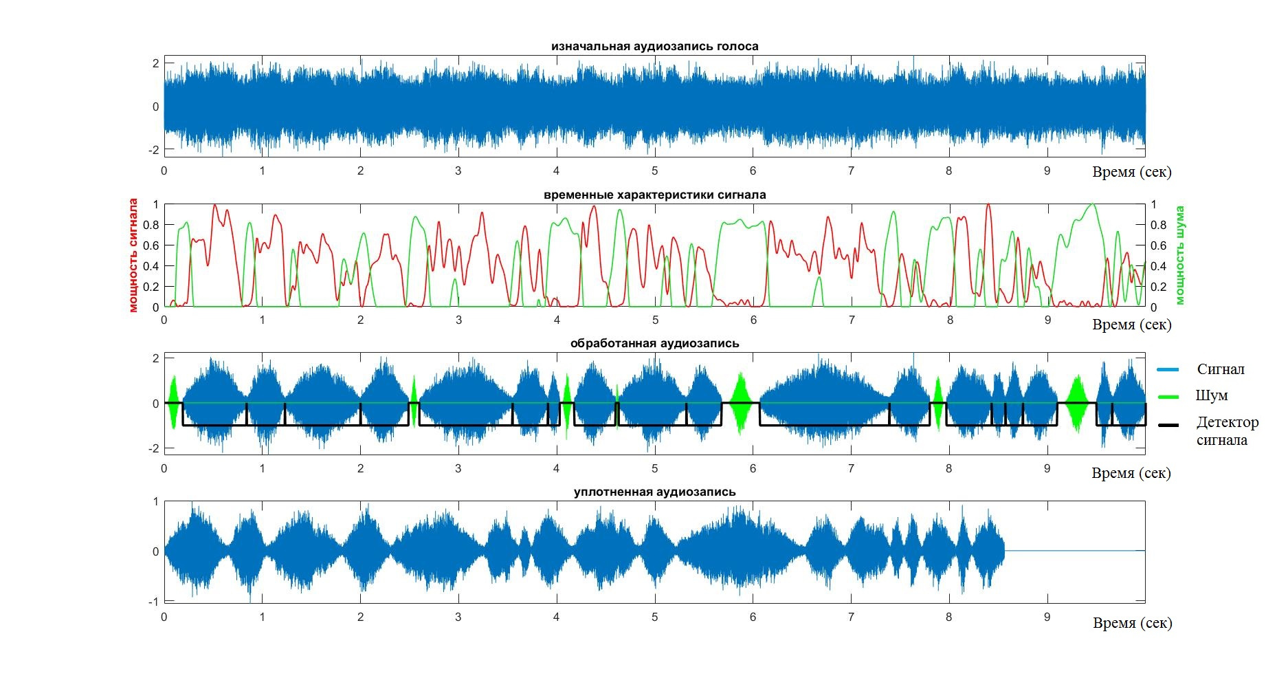
 %% create output sample array y = zeros(size(x)); phrase_space = zeros(size(x)); betta = 3; for iter = 1 : length(phrase) phrase_length = phrase(iter).start : phrase(iter).end; if (phrase(iter).voice) y(phrase_length) = x(phrase_length) .* kaiser(length(phrase_length), betta); phrase_space(phrase_length) = -1; else y(phrase_length) = zeros(size(phrase_length)); end if (0 < phrase(iter).end) phrase_space(phrase(iter).end) = 0; end end %% delete zero data for iter = length(phrase) : -1 : 1 phrase_length = phrase(iter).start : phrase(iter).end; if (~phrase(iter).voice) y(phrase_length) = []; end end 

At this point, the operation of the VAD system can be considered finished. At the output we have an array containing only the voice signal. In order to once again run through the stages of the algorithm, as well as to verify the adequacy of its work, you should pay attention to the following schedule.

• Audio is marked in blue.
• Red color - power of a speech signal
• Green - everything related to noise

Testing

In order to check the validity, accuracy and stability of the VAD system, the system was tested on about 20 audio recordings of various people. In all cases, testing took place on the eye and on the “ear” - it looked at the chart and listened to the condensed signal. A mistake was the omission of words or, on the contrary, the adoption of periods of calm.

After I made sure that the algorithm copes with its task for simple cases, I began to add different noise to the background.

In this case, being sure that in the noiseless case the algorithm works, I took it as a standard and found the Hamming distance between the indices of the standards and the test set. Thus, having received large reference and test sets, I made a statistical graph of the algorithm error (according to Hamming) depending on the SNR . Here the blue line indicates the average value, and the red line - the limits of the confidence interval.

Mfcc

To be honest, there is no MFCC here. I use this term because the goals and means of MFCC coincide with mine. In addition to that, the term is well established and its abbreviation takes only 4 letters. The difference from the main MFCC method is that in this case the inverse transformation into the time domain was not used for computational efficiency reasons, and also logarithmic decimation is used instead of the chalk-convolution.

You can read about MFCC here , here , here or here .

Logarithmic spectrum decimation

For the problem of logarithmic decimation, an array of a smaller number of points was created, the first and last elements of which are 1 and the maximum frequency, but all internal points are the result of an exponential function. Thus, choosing points for sampling from the created array and averaging the values ​​of the original function between points was allocated an array of much smaller dimension.

The idea is to create an array of indices, the value of which is logarithmically distributed over the whole space of indices of the original spectrum.

 function [ index_space ] = log_index_space( amount_point, input_length, decimation_speed ) index_space = exp(((0:(amount_point-1))./(amount_point-1)).*decimation_speed); index_space = index_space - index_space(1); index_space = index_space ./ index_space(end); index_space = round((input_length - 1) .* index_space + 1); end 

After compiling the array of indices, the only thing that remains is to select the necessary points of the original spectrum and accumulate the average energy between the points.

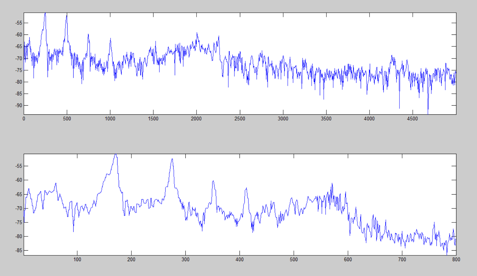
 function [ y ] = decimation_spectrum( freq_signal, index_space ) y = zeros(size(index_space)); min_value = min(freq_signal); freq_local = freq_signal - min_value; for iter = 2 : (length(index_space)-1) index_frame = index_space(iter - 1) : index_space(iter + 1); frame = freq_local(index_frame); if (4 < length(index_frame)) gw = gausswin(round(length(index_frame) / 2)); frame = filter(gw, 1, frame) ./ (round(length(index_frame)) / 4); end y(iter) = median(frame); end y(1) = mean(y); y(end) = y(end-1); y = y + min_value; end function [sample_spectr,log_space]=eject_spectr(sample_length,sample,fs,band_pass) %% set parameters band_start = band_pass(1); band_stop = band_pass(2); decimation_speed = 2.9; amount_point = 800; %% create spaces spectrum_space = 0 : fs/length(sample) : (fs/2) - (1/length(sample)); spectrum_space = spectrum_space(spectrum_space <= band_stop); sample_index_space = ... log_index_space(amount_point, length(spectrum_space), decimation_speed); %% create spectral density sample_spectr = 10*log10(abs(fft(sample,length(sample))) ./ (length(sample)*sample_length)); sample_spectr = sample_spectr(1 : length(spectrum_space)); sample_spectr = decimation_spectrum( sample_spectr, sample_index_space ); end 

An example of logarithmic decimation is presented below, where the upper graph is a logarithmic spectrum from 0 to 5000 Hz containing more than 16,000 points, and the lower one is a dedicated array of the main components of 800 points.

Building LogLog Spectrograms

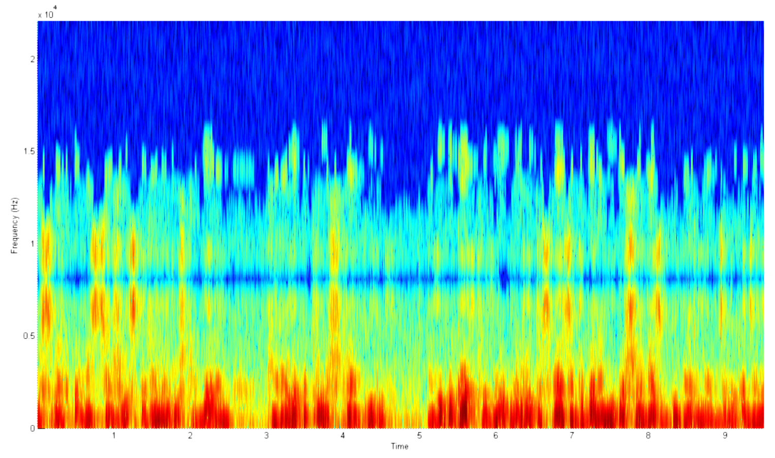
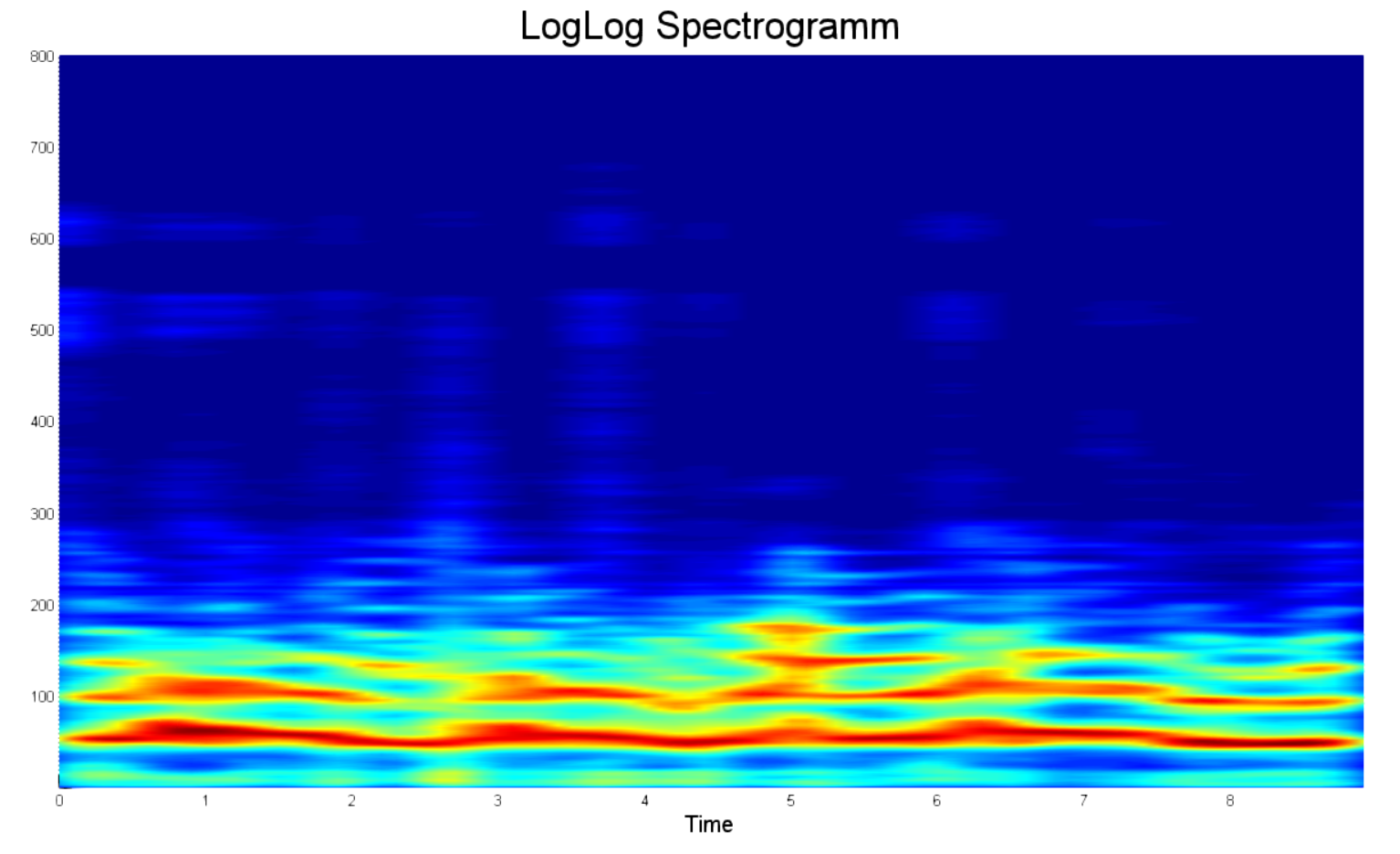
What are we talking about? What are all these efforts for? Why it is impossible to build a normal spectrogram using the matlab in one line and not to bathe with everything that was said earlier? But you can not, and here's why. The example below shows a typical voice spectrogram. What are the shortcomings in it?

• A huge number of points. No, there are a lot of them. So much so that my computer ran out of RAM when trying to build a 15-second spectrogram.
• Most of the information is about noise. Why do I need a 20kHz spectrum if no normal person ever speaks with such frequency?
• From 2.5 to 3 seconds and from 4.5 to 5 seconds there is no voice activity. This is noise. In addition, it is in the target frequency zone, and therefore may have a disastrous effect on the classification system in the future.
• There is no clear absolute power scale. Since audio recordings can be of different loudness, the final power in the spectrum can be very different even for the same person at different times.
• Not logarithmic magnitude. The loudness of a human voice, as well as the resolution of our hearing, is logarithmic in power.
• Not logarithmic frequency scale. In this regard, really useful information is concentrated only in a small part of the spectrum.

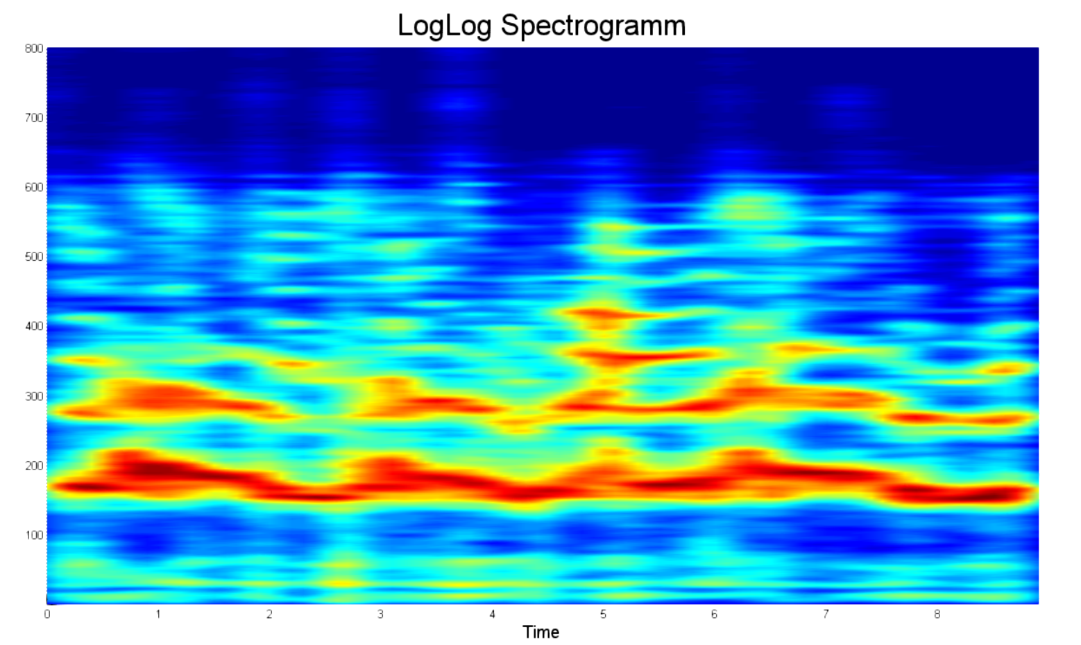
For a clearer comparison between the two spectrograms, here is an example of a processed LogLog spectrogram in the same frequency range as the one presented above. What strikes you in the first place?

• First, these are pronounced power peaks. Now you can distinguish the spectrum of two people just by sight.
• Secondly, there are no lull zones, they are cut out. Therefore, the duration is less.
• Thirdly, there are only 800 points on each frequency track. Yes, 800 points, not 20,000, as in the example above. Now you do not have to restart the computer when you accidentally messed with the duration.
• Fourth, the normalization of the power spectrum. It was decided to limit the spectrum power to 25 decibels. Anything that differed from the maximum by more than 25 decibels was considered to be zero.

At the same time, still most of the information is about noise. Therefore, it makes sense to cut the frequency sample at 8 kHz, as shown below.

 %% spetrogramm buffer_duration = 0.1; % in seconds overlap = 50; % in percent sample_size = round(buffer_duration * fs); buffer_size = round( ((1 + 2*(overlap / 100))*buffer_duration) * fs); time_space = 0 : sample_size/fs : length(y)/fs - 1/(fs); [~, log_space] = eject_spectr(buffer_size, x(1 : buffer_size), fs, band_pass); % array of power buffer samples db_range = 25; spectrum_array = zeros(length(time_space), length(log_space)); for iter = 1 : length(time_space) start_index = (iter - 1) * sample_size; start_index = max(round(start_index - (overlap / 100)*sample_size), 1); end_index = min(start_index + buffer_size, length(y)); phrase_space = start_index : end_index; buffer = y(phrase_space) ./ max(y(phrase_space)); buffer = buffer .* kaiser(length(buffer), betta); spectr = eject_spectr(buffer_size, buffer, fs, band_pass); spectr = max(spectr - (max(spectr) - db_range), 0); spectrum_array(iter, 1 : length(log_space)) = spectr; end spectrum_array = spectrum_array'; win_len = 11; win = fspecial('gaussian',win_len,2); win = win ./ max(win(:)); spectrum_array = filter2(win, spectrum_array) ./ (win_len*2); 

Statistical processing

What do we have at the moment? We have a 800-dimensional random process, the implementation of which depends on the spoken sound, mood and intonation of the speaker. However, the parameters of the process itself depend solely on the physical parameters of the speaker’s voice path and are therefore constant. The main question is how many of these parameters, and how to evaluate them.

"Yes, the center will come with you"

Why not present each of $$$800$processes as a sum $$$k$different Gaussian processes? Thus it turns out just $$$800 * k$various processes. For this approach, even came up with the name - GMM .

So, it remains to deal only with what is this $$$k$. Take the spectrogram, build a histogram on it and voila:

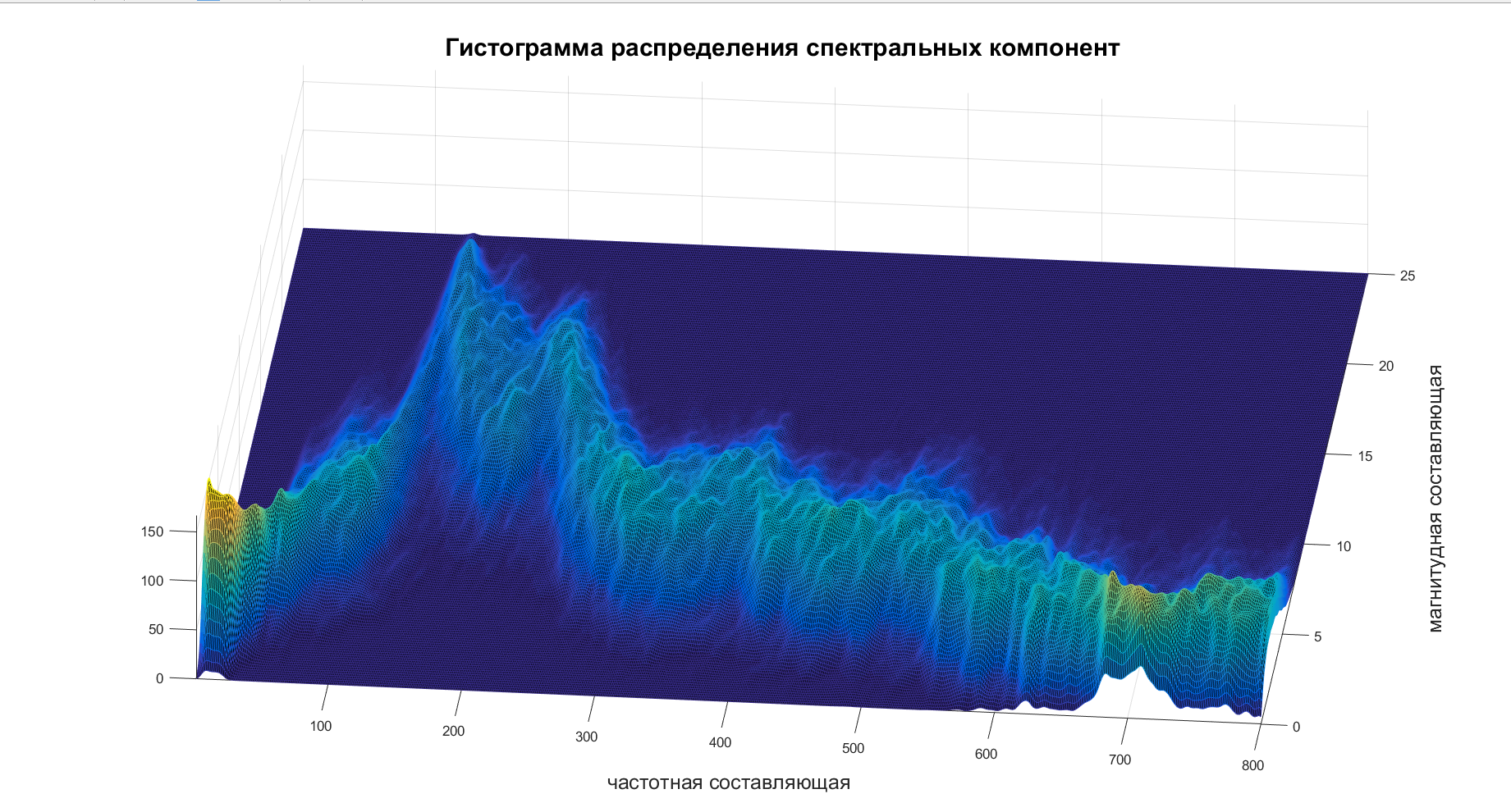
After viewing several such histograms, my laziness celebrated a decisive victory and set $$$k = 1$. After that, she proposed to score on the compilation of a covariance matrix of the connection of different frequencies and consider each frequency component to be independent, which is not true. Laziness - she is.

Now it remains only to calculate the estimates of MO and MSE for each frequency component, and then combine them into one vector of main components.

 std_spectr = std(spectrum_array, 0, 1); mean_spectr = mean(spectrum_array, 1); principal_component = cat(2, mean_spectr, std_spectr); 

Conclusion

In the technique of biometric authentication, static methods greatly exceed the dynamic in accuracy and speed of reaction. However, despite this, dynamic methods have a number of advantages that are purely practical and do not affect the recognition process, but may be the most significant for the customer.

When implementing systems on dynamic features such advantages can be:

• low cost of equipment
• low noise sensitivity
• Ease of registering a person and retrieving data.