Calculation of the weight spectrum of a linear subspace in Wolfram Mathematica

The process of calculating the weight spectrum
Root cause
This article owes its appearance to one rather long-standing question that was asked in the Wolfram Mathematica Russian-speaking support group. However, the answer to it greatly grew and eventually began to live an independent life, and even got its own problems. As is clear from the title of the article, the task was devoted to calculating the weight spectrum, and therefore it directly relates to discrete mathematics and linear algebra. It also shows the solution in the programming language Wolfram Language. Despite the fact that the essence of the problem is very simple (for simple basic vectors, it is completely solved in the mind), much more interesting is the process of optimizing the algorithm for finding the weight spectrum. The authors are of the opinion that the problem considered in this article and the ways to solve it very well show how compilation and parallelization are used in Wolfram techniques. Thus, the main goal is to show one of the effective ways to accelerate Mathematica code.
Wording
We quote the original formulation of the problem:
a) Let's call a vector a string of bits (values 0 or 1) of a fixed length N: that is, just 2 N different vectors are possible.
b) Introduce the addition operation modulo 2 vectors (operation xor), which takes two vectors a and b to receive a vector a + b of the same length N.
c) Let the set A = {a i | i ∈ 1..K} of 0 ≤ K ≤ 2 N vectors. Let's call it generating: by adding a i of the set A, we can get 2 K vectors of the form ∑ i = 1..K b i a i , where b i is equal to either 0 or 1.
')
d) The weight of a vector is the number of single (non-zero) bits in the vector: that is, the weight is a natural number from 0 to N.
It is required for the given generating sets of vectors and the number N to construct a histogram (spectrum) of the number of different vectors by their weight.
Input format:
Text file from a set of lines of the same length, one vector per line (characters 0 and 1 without separators).
Output Format:
A text file with a pair of values for the weight / number separated by a tab, one pair per line, sorted by the numerical value of the weight.
Manual solution
To begin with, we will try to solve the problem in our mind in order to understand the principle of calculating the weight spectrum. For this we will use vectors of minimal length. Then you just need to expand the algorithm for any number of vectors and any dimension. Let given a basis of two vectors of two elements in each:
basis = {{0, 1}, {1, 1}} Since there are only two vectors, all possible linear combinations and, accordingly, combinations of values of b i will be 2 K , where K is the number of basis vectors. We get 4 of the following linear combinations:
mod2(0 * {0, 1}, 0 * {1, 1}) = {0, 0} mod2(0 * {0, 1}, 1 * {1, 1}) = {1, 1} mod2(1 * {0, 1}, 0 * {1, 1}) = {0, 1} mod2(1 * {0, 1}, 1 * {1, 1}) = {1, 0} Here it is assumed that the addition function modulo two is already properly defined. It turned out four vectors, the dimension of each is equal to two. To finally calculate the spectrum you just need to count the number of units in each resulting vector, that is:
sum({0, 0}) = 0 sum({1, 1}) = 2 sum({0, 1}) = 1 sum({1, 0}) = 1 Calculate the number of entries in the resulting list of each weight. And then, according to the requirements of the task, the result should look like this:
{{0, 1}, {1, 2}, {2, 1}} 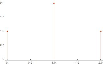
The implementation of a simple algorithm in Wolfram Mathematica
So, now we’ll try to record and automate everything that was done in our mind with the help of Wolfram Language. To begin with, let's create a function that performs modulo-2 addition (as it was said in the problem statement):
(* *) mod2[b1_Integer, b2_Integer] := Mod[b1 + b2, 2] (* *) mod2[b1_Integer, b2__Integer] := mod2[b1, mod2[b2]] (* - *) Attributes[mod2] := {Listable} The next function should take as input a list of vectors and a list of coefficients b i - a vector whose length is equal to the number of vectors in the basis. Returning a vector of the same dimension as the elements of the basis is a linear combination.
(* *) combination[basis: {{__Integer}..}, b: {__Integer}] /; Length[basis] == Length[b] := Apply[mod2, Table[basis[[i]] * b[[i]], {i, 1, Length[b]}]] Now you need to get a list of all possible sets of coefficients b i . Obviously, their number is 2 K , and all possible sets are simply writing all the numbers from 0 to 2 K -1 in binary representation. Then the list of all possible linear combinations can be obtained as follows:
linearCombinations[basis: {{__Integer}..}] := With[{len = Length[basis]}, Table[combination[basis, IntegerDigits[i, 2, len]], {i, 0, 2^len - 1}] ] The result of the function above is a list of 2 K vectors. All we have to do is calculate the weight of each vector in this list, and then count the number of meetings of each weight:
weightSpectrum[basis: {{__Integer}..}] := Tally[Map[Total, lenearCombination[basis]]]; Check how it will work. Create a basis from the list of random vectors and calculate the weight spectrum:
(* *) basis = RandomInteger[{0, 1}, {6, 6}] ws = weightSpectrum[basis] ListPlot[ws, PlotTheme -> "Web"] (* Out[..] := {{0, 0, 1, 1, 1, 0}, {1, 0, 0, 0, 0, 1}, {1, 1, 0, 1, 0, 1}, {1, 0, 0, 1, 1, 0}, {1, 0, 0, 0, 1, 1}, {0, 1, 0, 1, 1, 1}} Out[..]:= {{0, 1}, {4, 15}, {3, 20}, {2, 15}, {1, 6}, {5, 6}, {6, 1}} *) 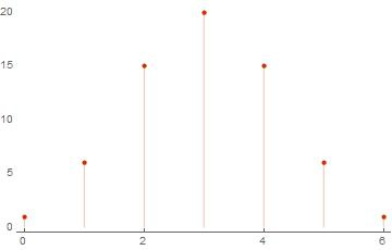
But what will happen if you try to calculate all the same, but for more vectors? We use the AbsoluteTiming [] function and see how the calculation time behaves itself depending on the size of the basis.
basisList = Table[RandomInteger[{0, 1}, {i, 10}], {i, 1, 15}]; timeList = Table[ {Length[basis], First[AbsoluteTiming[weightSpectrum[basis]]]}, {basis, basisList} ]; ListPlot[timeList, PlotTheme -> "Web", Joined -> True] 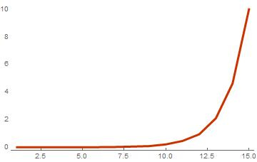
The dependence of the calculation time on the size of the basis for the same length of vectors
As can be seen in the resulting graph, the calculation time increases exponentially along with the addition of the number of vectors to the basis. It turns out that for a basis of 15 vectors, where 10 elements each, the calculation of the spectrum takes about 10 seconds. This calculation time is quite large, but there is nothing surprising in this, since it has already been said above that the number of linear combinations grows exponentially with the size of the basis, and hence the number of operations increases with the same speed. Another factor that lowers the computation speed is that the code is not optimal. Wolfram Language is an interpreted programming language and therefore is not initially considered to be fast enough, which means that standard functions will not give us maximum performance. To solve this problem, we use the compilation.
Using compiled functions
Compile in Brief
The syntax of this function is quite simple and very similar to Function . As a result, Compile always returns an "object" - a compiled function that can be applied to numeric values or lists of numbers. Compile does not support working with Wolfram Language strings, characters, or compound expressions (except expressions consisting of a List ). Below are some examples of creating compiled functions.
cSqr = Compile[{x}, x^2]; cSqr[2.0] (* Out[..] := 4.0 *) cNorm = Compile[{x, y}, Sqrt[x^2 + y^2]]; cNorm[3.0, 4.0] (* Out[..] := 5.0 *) cReIm = Compile[{{z, _Complex}}, {Re[z], Im[z]}]; cReIm[1 + I] (* Out[..] := {1.0, 1.0} *) cSum = Compile[{{list, _Real, 1}}, Module[{s = 0.0}, Do[s += el, {el, list}]; s]]; cSum[{1, 2, 3.0, 4.}] (* Out[..] := 10.0 *) All available options and more detailed examples can be found in the official documentation at the link above. Now let's go directly to the function for calculating the weight spectrum.
Compiling weight spectrum computations
As in the simple case, you can create some simple functions and then apply them in turn to get the result. And you can perform all operations in the body of just one function. Both that and other method can be quite realized. We will go the second way for the sake of diversity.
cWeightSpectrumSimple = Compile[ {{basis, _Integer, 2}}, Module[ { k = Length[basis], spectrum = Table[0, {i, 0, Last[Dimensions[basis]]}] }, Do[ With[ { (* 2^k - 1 *) weight = Total[Mod[Total[IntegerDigits[b, 2, k] * basis], 2]] + 1 }, (* spectrum . weight - 1 , . spectrum . , . *) spectrum[[weight]] = spectrum[[weight]] + 1 ], {b, 0, 2^k - 1} ]; Return[Transpose[{Range[0, Last[Dimensions[basis]]], spectrum}]] ] ] As always, we will conduct a small test of the correctness of this function. Similarly, we take a list of random bases with sizes from 2 to 15 vectors, where each vector consists of 10 elements and try to calculate the time at which the weight spectrum is calculated:
basisList = Table[RandomInteger[{0, 1}, {i, 10}], {i, 2, 15}]; timeList=Table[{Length[basis],First[AbsoluteTiming[cWeightSpectrumSimple[basis]]]},{basis,basisList}]; ListLinePlot[timeList, PlotTheme -> "Web"] 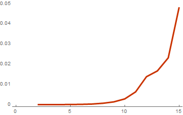
As can be seen from the last graph - the difference with the result from the previous part is huge. A small optimization of the algorithm in the form of an optimal weight calculation at the last stage and the use of compilation leads to an acceleration of 200 times! This result is interesting because, on the one hand, it shows Mathematica as a fairly fast language, when properly applied, and on the other, it once again proves that Mathematica is a slow language because of interpretability, if you do not know the intricacies of the internal workings of functions.
Gray code
About Gray Code
While thinking about how to solve the problem, a simple thought arose. If suddenly the next value of b i is zero, then there is generally no need to multiply the base vector by that number and add it. Those vectors that are multiplied with zero values do not change the result. At first it seemed like a great thought and it even worked. Indeed, during the iteration of the list elements b i just came out fewer vector addition operations. Then came the next idea. The subtraction and addition of vectors in the calculation of a linear combination is no different. This means that the following is feasible:
1 * {0, 1} + 0 * {1, 0} + 1 * {1, 1} == {0, 1} + {1, 1} {0, 1} + {1, 1} == {1, 0} -> {1, 0} + {1, 1} == {0, 1} That is, adding a vector to the intermediate sum is no different from subtracting. And then it all came together in a great idea! What if suddenly it turns out that in the cycle for the list b i the difference between the representation b k and b k + 1 is just a few bits? Then you can get a linear combination with the number k and add to it only those basic vectors whose index coincides with the numbers of the different bits between k and k + 1 . The result is a linear combination of k + 1 . And what if you go further? Suddenly it turns out that the difference between adjacent linear combinations in just one vector? If you build a direct sequence from 0 to 2 N -1 - then this is impossible. But suddenly you can mix and arrange these numbers in some other order? This, as it turned out, is called the Gray Code, a sequence of numbers, in which the difference between neighbors is only one digit. Wikipedia describes one of the infinite set of codes - the mirror Gray Code and the method for obtaining it. Below is an example of such a sequence:
| Decimal | Binary | Gray | Gray as decimal |
|---|---|---|---|
| 0 | 000 | 000 | 0 |
| one | 001 | 001 | one |
| 2 | 010 | 011 | 3 |
| 3 | 011 | 010 | 2 |
| four | 100 | 110 | 6 |
| five | 101 | 111 | 7 |
| 6 | 110 | 101 | five |
| 7 | 111 | 100 | four |
Use in compiled function
The use of compilation already significantly speeds up the calculation of the weight spectrum; now we will try to use the Gray code and optimize the addition of the linear combination vectors. Only it is necessary to understand how to calculate the position of the changed bit at each step. Fortunately, the 13th chapter of this book came to the rescue. Entirely calculate the linear combination is required only once at the very beginning. But, since it is precisely known that the first linear combination is a set of zeros, this will not be necessary. Considering the above, you can create an even more optimized function for calculating the weight spectrum:
WeightSpectrumLinearSubspaceGrayCodeEasy = Compile[{{basevectors, _Integer, 2}}, Module[{ n = Dimensions[basevectors][[-1]], k = Length[basevectors], s = Table[0, {n + 1}], currentVector = Table[0, {n}], (* {0, 0, ..}*) m = 0, l = 0 }, (* , 0 1 *) s[[1]] = 1; Do[ (* *) m = Log2[BitAnd[-1 - b, b + 1]] + 1; (* , *) currentVector = BitXor[currentVector, basevectors[[m]]]; (* *) l = Total[currentVector] + 1; s[[l]] = s[[l]] + 1, {b, 0, 2^k - 2} ]; (* Return *) s ], (* , *) RuntimeOptions -> "Speed", (*CompilationTarget -> "C",*) CompilationOptions -> {"ExpressionOptimization" -> True} ]; Here is an example of the result for a basis of 16 vectors with a dimension of 512:
basis = RandomInteger[{0, 1}, {16, 512}]; ListPlot[WeightSpectrumLinearSubspaceGrayCodeEasy[basis], PlotTheme -> "Web", PlotRange -> All, Filling -> Bottom] 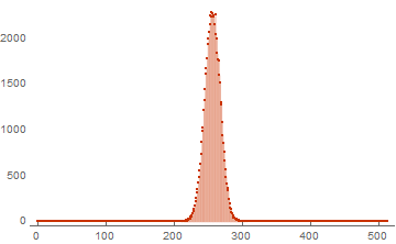
As a result, a one-dimensional list of weights is returned. This type of list is also quite correct, as it is easy to bring it to the view from the previous part. The first element corresponds to the frequency of meeting the vector of zero weight. The latter is the frequency of the meeting of the vector of units. We use the same code to test performance:
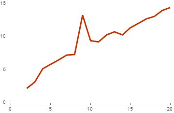
basisList = Table[RandomInteger[{0, 1}, {i, 10}], {i, 2, 15}]; timeList=Table[{Length[basis],First[AbsoluteTiming[WeightSpectrumLinearSubspaceGrayCodeEasy[basis]]]},{basis,basisList}]; ListLinePlot[timeList, PlotTheme -> "Web"] 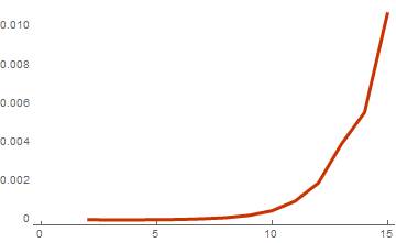
Calculation time on basis size
As a result, for the last basis from the list of 15 vectors, the computation speed increased by another 5 times. But this is a slightly misleading result. To understand how much efficiency has increased it is necessary to calculate the ratio of the calculation time for the last two functions:
basisList = Table[RandomInteger[{0, 1}, {i, 10}], {i, 2, 20}]; timeList=Table[{ Length[basis], First[RepeatedTiming[cWeightSpectrumSimple[basis]]] / First[RepeatedTiming[WeightSpectrumLinearSubspaceGrayCodeEasy[basis]]] }, {basis,basisList} ]; ListLinePlot[timeList, PlotTheme -> "Web"] 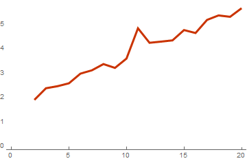
The ratio of the spectrum calculation time using gray code and without
From this graph it becomes clear that in fact this algorithm lowered the complexity of computations by one power. And this will be the more noticeable and more efficient the larger the dimension of the vectors in the basis. This result is obtained if the basis consists of vectors with dimension 128:
Parallelization
How to calculate something in Mathematica in parallel
Mathematica has a small set of functions that can perform asynchronous computations on different cores. Only now it is necessary to define with terminology. After all, a running process that represents something similar to a virtual machine in Mathematica is also called a kernel, i.e. Kernel. The Mathematics Core is an interactive execution environment operating in interpreter mode. Each core takes necessarily one process in the system. Threads in the usual sense of the language does not implement. Accordingly, you need to understand that the kernels in standard use will not have shared memory. Basically, all functions of this type begin on Parallel . The easiest way to find something asynchronously:
ParallelTable[i^2,{i, 1, 10}] (*Out[..] := {1, 4, 9, 16, 25, 36, 49, 64, 81, 100}*) A number of functions work in a similar way:
ParallelMap , ParallelDo , ParallelProduct , ParallelSum , ...
There are several ways to verify that this was not actually done on one core. This is how you can get all the running kernels:
Kernels[] (* Out[..] := {"KernelObject"[1, "local"], ... , "KernelObject"[N, "local"]} *) The list will contain all currently running processes. At the same time, they should also be displayed in the task manager.

Two of the six processes are responsible for running the session, and the rest are local kernels, which are used for parallel computing. In this case, by default the number of local cores of Mathematica coincides with the number of physical cores of the processor. But no one bothers to create more. This is done using LaunchKernels [n] . As a result, an additional n cores are launched. And the number of available processor cores can be viewed in the $ KernelCount variable.
The functions listed at the beginning produce an automatic distribution of tasks among the processes. However, there is a way to independently send code to run on a specific kernel. This is done using ParallelEvaluate + ParallelSubmit :
ParallelEvaluate[$KernelID, Kernels[][[1 ;; 4 ;; 2]]] (* Out[..] := {1, 3}*) This set of functions will be enough to be able to parallelize the task of calculating the weight spectrum.
The division of the main loop into parts
Check whether the calculations actually occur in parallel. For four physical cores, this means that the calculation on all four cores will take as much time as on one:
basis = RandomInteger[{0, 1}, {24, 24}]; AbsoluteTiming[WeightSpectrumLinearSubspaceGrayCodeEasy[basis];][[1]] AbsoluteTiming[ParallelEvaluate[WeightSpectrumLinearSubspaceGrayCodeEasy[basis]];][[1]] (* Out[..] := 6.518... Out[..] := 8.790...*) There is a time difference, but not fourfold. So with this, everything is fine. The next step is to figure out how to divide the task into several parts. The most logical and effective is to compute only part of the linear combinations on each core. That is, as a result, each core returns a partial spectrum. But how to divide the list b i . After all, it is not a direct sequence! In this case, a function is needed that calculates the value from the Gray Code sequence by index. This is done like this:
grayNum[basis_List, index_Integer] := IntegerDigits[BitXor[index, Quotient[index, 2]], 2, Length[basis]] Grid[Table[{i, Row[grayNum[{{0, 0}, {0, 1}, {1, 1}}, i]]}, {i, 0, 7}]] | index | code |
|---|---|
| 0 | 000 |
| one | 001 |
| 2 | 011 |
| 3 | 010 |
| four | 110 |
| five | 111 |
| 6 | 101 |
| 7 | 100 |
Now we modify the compiled function so that it considers only a partial spectrum in a certain range of indices of linear combinations:
WeightSpectrumLinearSubspaceGrayCodeRange = Compile[{{basis, _Integer, 2}, {range, _Integer, 1}}, Module[{ n = Dimensions[basis][[-1]], k = Length[basis], s = Table[0, {n + 1}], currentVector = Table[0, {i, 1, Length[basis[[1]]]}], m = 0, l = 0 }, (* *) If[range[[1]] =!= 0, currentVector = Mod[Total[basis Reverse[IntegerDigits[BitXor[range[[1]], Quotient[range[[1]] + 1, 2]], 2, k]]], 2]; ]; Mod[Total[basis IntegerDigits[BitXor[range[[1]] - 1, Quotient[range[[1]] - 1, 2]], 2, k]], 2]; s[[Total[currentVector] + 1]] = 1; Do[ m = Log2[BitAnd[-1 - b, b + 1]] + 1; currentVector = BitXor[currentVector, basis[[m]]]; l = Total[currentVector] + 1; s[[l]] = s[[l]] + 1, {b, First[range], Last[range] - 1, 1} ]; (* Return *) s ], (* , *) RuntimeOptions -> "Speed", (*CompilationTarget -> "C",*) CompilationOptions -> {"ExpressionOptimization" -> True} ]; That is, if earlier the function counted all combinations with numbers from 0 to 2 N -1, then now this range can be set manually. Now we will try to figure out how to divide this very range into equal parts depending on the number of available cores:
partition[{i1_Integer, iN_Integer}, n_Integer] := With[{dn = Round[(iN - i1 + 1)/n]}, Join[ {{i1, i1 + dn - 1}}, Table[{dn * (i - 1), i * dn - 1}, {i, 2, n - 1}], {{(n - 1) * dn, iN}} ] ] Now, in order to calculate the full spectrum in such a way, it is necessary to calculate it on each of the segments, and then add all the results. For example:
WeightSpectrumLinearSubspaceGrayCodeEasy[{{1, 1}, {1, 1}, {1, 1}}] WeightSpectrumLinearSubspaceGrayCodeRange[{{1, 1}, {1, 1}, {1, 1}}, {0, 3}] WeightSpectrumLinearSubspaceGrayCodeRange[{{1, 1}, {1, 1}, {1, 1}}, {4, 7}] (* Out[..] := {4, 0, 4} = Out[..] := {2, 0, 2} + Out[..] := {2, 0, 2} *) The final step is to send these calculations to different kernels:
WeightSpectrumLinearSubspaceGrayCodeParallel[basis: {{__Integer}..}] := With[{ kernels = (If[Kernels[] === {}, LaunchKernels[]]; Kernels[]), parts = partition[{0, 2^Length[basis] - 1}, Length[Kernels[]]] }, Total[WaitAll[Table[ ParallelEvaluate[ParallelSubmit[WeightSpectrumLinearSubspaceGrayCodeRange[basis, parts[[$KernelID]]]], kernel], {kernel, kernels} ]]] ] Here you need to clarify. Such a combination of ParallelEvaluate + ParallelSubmit in order to manually control which core will run on which part of the code. ParallelEvaluate generally cannot figure out how to properly execute asynchronous code and ultimately does it in one stream. In the general case, ParallelSubmit does not allow you to specify the correct core, but selects it automatically.
Check if this feature works:
ListPlot[WeightSpectrumLinearSubspaceGrayCodeParallel[RandomInteger[{0, 1}, {16, 128}]], PlotRange -> All, PlotTheme -> "Web", Filling -> Bottom] 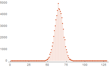
And as usual we will look at the difference in the speed of calculations. Since a laptop with a 4-core processor is used, an acceleration of about 4 times is expected. Plus, we must take into account the time for the division of tasks and the addition of the final result:
basis = RandomInteger[{0, 1}, {20, 1024}]; AbsoluteTiming[WeightSpectrumLinearSubspaceGrayCodeEasy[basis];] AbsoluteTiming[WeightSpectrumLinearSubspaceGrayCodeParallel[basis];] (* Out[..] := {5.02..., Null} Out[..] := {1.5....., Null} *) Naturally, with a larger number of processor cores, the difference will be more noticeable. Now we will try to calculate the spectrum of the base more. I wonder how long it will take? Suppose we assume to increase the size of the basis until one calculation takes more than a minute:
spectrums = Block[{i = 1, basis, res}, Reap[ While[True, i++; basis = RandomInteger[{0, 1}, {i, i}]; Sow[res = AbsoluteTiming[WeightSpectrumLinearSubspaceGrayCodeParallel[basis]]]; If[res[[1]] > 60, Break[]] ] ][[-1, -1]]] ListPlot[spectrums[[-1, -1]], PlotLabel->Row[{"basis len: ", Length[spectrums] + 1, "; time: ", Round[spectrums[[-1, 1]], 0.01], " sec"}], Filling->Bottom,PlotTheme->"Web",PlotRange->All] 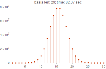
The picture clearly shows that in a minute and a half the function can calculate the spectrum for a basis of 29 vectors. This is a very good result, given that the very first option, which does not use compilation, is gray code, parallelization is hardly capable of all the same in a reasonable time. The computation time will be thousands of times longer if even for 15 vectors with dimension 10 the calculation took more than 10 seconds.
Conclusion
I do not know who and where applies all that was described in the article. Wikipedia says the Gray Code has a practical purpose. I also know that the calculation of spectra is often associated with encryption and some other problems of linear algebra. , , : , . , .
Source: https://habr.com/ru/post/336350/
All Articles