How to make a project on the recognition of handwritten numbers with additional training online. Hyde for not quite beginners
Hi, Habr! Recently, machine learning and data science in general are becoming increasingly popular. New libraries are constantly appearing and quite a bit of code may be required to train machine learning models. In such a situation, you can forget that machine learning is not an end in itself, but a tool for solving a problem. It is not enough to make a working model, it is equally important to present the analysis results qualitatively or to make a working product.
 I would like to talk about how I created a project for recognizing handwritten input of numbers with models that are trained on user-drawn numbers. Two models are used: simple neural network (FNN) on pure numpy and convolutional network (CNN) on Tensorflow. You can learn how to do the following from practically nothing:
For a full understanding of the project, it is advisable to know how deep learning works for image recognition, have a basic knowledge of Flask and understand a bit about HTML, JS and CSS.
After graduating from the Faculty of Economics of Moscow State University, I worked for 4 years in IT consulting in the field of implementation and development of ERP systems. It was very interesting to work, over the years I learned a lot of useful things, but over time it came to the realization that this is not mine. After much deliberation, I decided to change the scope of activities and move to machine learning (not because of hype, but because I really became interested). For this, he quit and worked for about half a year, independently studying programming, machine learning and other necessary things. After that, with difficulty, but still found work in this direction. I try to develop and improve my skills in my free time.
')
A few months ago, I passed a Yandex and MIPT specialization on Coursera. She has her own team in Slack, and in April there the group organized itself for passing the Stanford course cs231n. How this happened is a separate story, but more to the point. An important part of the course is an independent project (40% of the assessment for students), which provides complete freedom of action. I did not see the point of doing something serious and then writing about this article, but still my soul asked me to complete the course adequately. Around this time, I came across a website where you can draw a number and two grids on Tensorflow instantly recognize it and show the result. I decided to do something similar, but with my own data and models.
Here I will talk about what and how I did to implement the project. The explanations will be sufficiently detailed so that you can repeat what has been done, but I will briefly describe or skip some basic things.
Before you start something big, it is worth it to plan something. Along the way, new details will be found out and the plan will have to be corrected, but some initial vision simply must be.
Almost half of all the time spent on the project took me to collect data. The fact is that I was not very familiar with what had to be done, so I had to move by trial and error. Naturally, it was not the drawing itself that was difficult, but the creation of a site on which it would be possible to draw numbers and save them somewhere. For this, I needed to get to know Flask better, dig into Javascript, get acquainted with the Amazon S3 cloud and learn about Heroku. I describe all this in sufficient detail so that it can be repeated, having the same level of knowledge that I had at the beginning of the project.
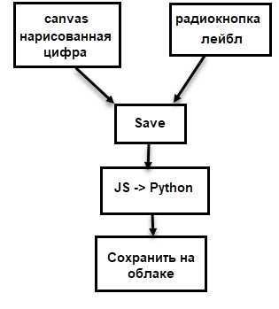
Previously, I drew such a scheme:
The data collection itself took several days, well, or several hours of pure time. I drew 1000 numbers, about 100 each (but not exactly), tried to draw in different styles, but, of course, I could not cover all the possible variants of handwriting, which, however, was not the goal.
The first version of the site looked like this:

It had only the most basic functionality:
So, now more about all this. Especially for the article I made a minimally working version of the site, by the example of which I will tell you how to do the above: Site Code
Note: if the site has not been opened for a long time, then its launch can take up to 20-30 seconds - the costs of the free version of hosting. This situation is relevant for the full version of the site.
Flask - Python framework for creating websites. The official site has a great introduction . There are different ways to use Flask to receive and transfer information, so in this project I used AJAX. AJAX allows for “background” data exchange between the browser and the web server, this allows you not to reload the pages every time you transfer data.

All files used in the project can be divided into 2 unequal groups: the smaller part is necessary for the application to work on Heroku, and all the others are directly involved in the work of the site.
HTML files should be stored in the folder “template”, at this stage it was enough to have one. In the header of the document and at the end of the body tag are links to js and css files. These files themselves must be in the “static” folder.
Now more about how drawing on canvas and saving the picture works.
Canvas is a two-dimensional HTML5 element for drawing. The image may be drawn by a script or the user may be able to draw using the mouse (or by touching the touch screen).
Canvas is defined in HTML as follows:
Before that, I was not familiar with this element of HTML, so my initial attempts at drawing ability were unsuccessful. After a while, I found a working example and borrowed it (the link is in my draw.js file).
There are 4 more elements in the interface:
Canvas content is cleared, and it is filled with white. Also, the status becomes empty.
Immediately after pressing the button, the value of “connecting ...” is displayed in the status field. The image is then converted to a text string using the base64 encoding method. The result is as follows:
Then I take the value of the active radio button (by name = 'action' and as
Finally, the AJAX request sends the encoded image and label to the python, and then receives a response. I spent quite a lot of time trying to make this construction work, I will try to explain what is happening in each line.
First, the type of request is specified - in this case “POST”, that is, the data from JS is transferred to the python script.
"/ hook" is where data is transferred. Since I use Flask, I can specify "/ hook" as the URL in the desired decorator, and this will mean that the function in this decorator will be used when a POST request is sent to this URL. More on this in the section about Flask below.
Finally,
To distract, I want to talk about a small problem that arose at the beginning of the project. For some reason, this basic site for image processing was loaded for about a minute. I tried to minimize it, leaving just a few lines - nothing helped. As a result, thanks to the console, it was possible to identify the source of the brakes - antivirus.

It turned out that Kaspersky inserts his script into my site, which led to inadequately long loading. After disabling the option, the site began to load instantly.
Now let's move on to how data from an AJAX request gets into python, and how the image is saved.
There are many guides and articles on working with Flask, so I’ll just briefly describe the basic things, pay special attention to the lines without which the code does not work, and, of course, I’ll tell you about the rest of the code that is the basis of the site.
And now you can talk about how the Amazon cloud works and what you can do with it.
Python has two libraries for working with the Amazon cloud: boto and boto3. The second is newer and better supported, but so far some things are more convenient to do using the first.
Now actually about the code. For now, it’s about how to save files on Amazon. About receiving data from the cloud will be discussed later.
The first step is to create a connection to the cloud. To do this, you must specify the Access Key ID, Secret Access Key and Region Host. We have already generated the keys, but it is dangerous to indicate them explicitly. This can be done only when testing the code locally. I hit the code on github a couple of times with openly specified keys - they were stolen for a couple of minutes. Do not repeat my mistakes. Heroku provides the ability to store keys and refer to them by name - more on this below. The region host is the endpoint value from the region label.
After that, you need to connect to the bucket - here it is already quite possible to specify the name directly.
It's time to talk about how to place a website on Heroku. Heroku is a multi-language cloud platform that allows you to quickly and conveniently deploy web applications. It is possible to use Postgres and a lot of interesting things. Generally speaking, I could store images using Heroku resources, but I need to store different types of data, so it was easier to use a separate cloud.
Heroku offers several price plans, but for my application (including the full-fledged one, not this small one), the free one is enough. The only minus is that the application “falls asleep” after half an hour of activity and at the next launch it can spend 30 seconds to “wake up”.
You can find a lot of guides on deploying applications on Heroku (here is a link to the official one ), but most of them use the console, and I prefer to use interfaces. Besides, it seems to me much easier and more convenient.
Now you can run the application and work with it. This completes the site description for data collection. The following discussion focuses on data processing and the next stages of the project.
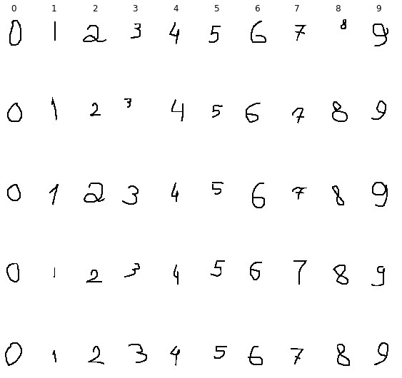
I save the drawn images as pictures in the original format, so that you can always look at them and try different processing options.
Here are some examples:
The idea of image processing for my project is as follows (similar to mnist): the drawn figure is scaled to fit in a 20x20 square, keeping the proportions, and then placed in the center of a white square 28x28 in size. The following steps are necessary for this:
It is obvious that 1000 images are not enough for training the neural network, and in fact some of them need to be used for model validation. — , . , , . .
, . 2020 . 4 — 4 .
. , — 30 ; 5 , 12 . , 12 6.
:
800 * 24 = 19200 200 . .
feed forward neural net. , cs231n, .
:
:
:
, loss , :

— . , , — , . . , , . , , , .
, . . learning rate, regularization, , -; , . .
, , , - . , , learning rate . . - , : , 1 . 1 24 , - . 24.
MNIST, MNIST.
:

, ~10 , .
, , MNIST . , , MNIST . CNN Tensorflow MNIST . MNIST 99%+ ( ), : 78.5% 63.35% . , MNIST , MNIST.
, :
. , .
:
.
. :
, — , learning rate.
learning rate . 0.1, 24 0.1 x (0.95 ^ 24). , — 800 . , . 0.1 x (0.95 ^ 24) / 32. , .
, FNN , CNN, , CNN, .
CNN cs231n Tenforlow MNIST, .

Tensorflow, , FNN numpy.
:
MNIST TF :
, FNN, - , :
CNN FNN, -. - , CNN , . , :

:
, , ~100 .
CNN , FNN: , 1 , -3 .
learning rate. 0.00001, 100 . , . , .
( ). -, , bootstrap. : html css, js . , , .
. :

main.py , functions.py .
«» , . FNN — ,
, tmp ( , ). , Amazon. , load_weights_amazon
Amazon : , ( , ,
Tensorflow , . , Tensorflow .
JS Python
4 . FNN , .
CNN , — . .
4 . ?
JS , — .
:
. :
JS / :
, , , .
23 « » . . , , ( ). , , , , « ». .
— . 2 : , ; mozilla . , , , .
— , / ( , , ), , «» .
: . , , 2,5 ( , ). … :

.
~ , ( slack ODS) . , , .
. . . . . , , data science , .
I would like to talk about how I created a project for recognizing handwritten input of numbers with models that are trained on user-drawn numbers. Two models are used: simple neural network (FNN) on pure numpy and convolutional network (CNN) on Tensorflow. You can learn how to do the following from practically nothing:- create a simple website using Flask and Bootstrap;
- place it on the Heroku platform;
- realize saving and loading of data using the Amazon s3 cloud;
- build your own dataset;
- train machine learning models (FNN and CNN);
- make the possibility of additional training of these models;
- make a website that can recognize drawn images;
For a full understanding of the project, it is advisable to know how deep learning works for image recognition, have a basic knowledge of Flask and understand a bit about HTML, JS and CSS.
Something about me
After graduating from the Faculty of Economics of Moscow State University, I worked for 4 years in IT consulting in the field of implementation and development of ERP systems. It was very interesting to work, over the years I learned a lot of useful things, but over time it came to the realization that this is not mine. After much deliberation, I decided to change the scope of activities and move to machine learning (not because of hype, but because I really became interested). For this, he quit and worked for about half a year, independently studying programming, machine learning and other necessary things. After that, with difficulty, but still found work in this direction. I try to develop and improve my skills in my free time.
')
The origin of the idea
A few months ago, I passed a Yandex and MIPT specialization on Coursera. She has her own team in Slack, and in April there the group organized itself for passing the Stanford course cs231n. How this happened is a separate story, but more to the point. An important part of the course is an independent project (40% of the assessment for students), which provides complete freedom of action. I did not see the point of doing something serious and then writing about this article, but still my soul asked me to complete the course adequately. Around this time, I came across a website where you can draw a number and two grids on Tensorflow instantly recognize it and show the result. I decided to do something similar, but with my own data and models.
Main part
Here I will talk about what and how I did to implement the project. The explanations will be sufficiently detailed so that you can repeat what has been done, but I will briefly describe or skip some basic things.
Project planning
Before you start something big, it is worth it to plan something. Along the way, new details will be found out and the plan will have to be corrected, but some initial vision simply must be.
- For any machine learning project, one of the fundamental issues is the question of what data to use and where to get it. Dataset MNIST is actively used in the tasks of recognition of numbers, and that is why I did not want to use it. On the Internet, you can find examples of such projects, where models are trained on MNIST (for example, the one mentioned above ), but I wanted to do something new. And finally, it seemed to me that many of the figures in MNIST are far from reality - when I looked at dataset, I came across many such options that are difficult to imagine in reality (if only a person has a really creepy handwriting). Plus drawing numbers in the browser with a mouse is somewhat different from writing them with a pen. As a result, I decided to build my own dataset;
- The next (or rather simultaneous) step is to create a site for data collection. At that time I had basic knowledge of Flask, as well as HTML, JS and CSS. That's why I decided to create a website on Flask, and Heroku was chosen as the hosting platform, as it allows you to quickly and easily capture a small website;
- Next was to create the models themselves, which should do the main work. This stage seemed the easiest, since after cs231n there was sufficient experience in creating neural network architectures for image recognition. Previously I wanted to make several models, but later I decided to dwell on two - FNN and CNN. In addition, it was necessary to make it possible to validate these models; I already had some ideas on this subject;
- After preparing the models, you should give the site a decent look, somehow display the predictions, give an opportunity to evaluate the correctness of the answer, describe the functionality a little and do a number of other small and not so great things. At the planning stage, I did not spend much time thinking about it, I just made a list;
Data collection
Almost half of all the time spent on the project took me to collect data. The fact is that I was not very familiar with what had to be done, so I had to move by trial and error. Naturally, it was not the drawing itself that was difficult, but the creation of a site on which it would be possible to draw numbers and save them somewhere. For this, I needed to get to know Flask better, dig into Javascript, get acquainted with the Amazon S3 cloud and learn about Heroku. I describe all this in sufficient detail so that it can be repeated, having the same level of knowledge that I had at the beginning of the project.
Previously, I drew such a scheme:
The data collection itself took several days, well, or several hours of pure time. I drew 1000 numbers, about 100 each (but not exactly), tried to draw in different styles, but, of course, I could not cover all the possible variants of handwriting, which, however, was not the goal.
Creating the first version of the site (for data collection)
The first version of the site looked like this:
It had only the most basic functionality:
- canvas for drawing;
- radio buttons for label selection;
- buttons for saving images and cleaning canvas;
- the field in which the save was written successfully;
- saving pictures on the Amazon cloud;
So, now more about all this. Especially for the article I made a minimally working version of the site, by the example of which I will tell you how to do the above: Site Code
Note: if the site has not been opened for a long time, then its launch can take up to 20-30 seconds - the costs of the free version of hosting. This situation is relevant for the full version of the site.
Flask in brief
Flask - Python framework for creating websites. The official site has a great introduction . There are different ways to use Flask to receive and transfer information, so in this project I used AJAX. AJAX allows for “background” data exchange between the browser and the web server, this allows you not to reload the pages every time you transfer data.
Project structure
All files used in the project can be divided into 2 unequal groups: the smaller part is necessary for the application to work on Heroku, and all the others are directly involved in the work of the site.
HTML and JS
HTML files should be stored in the folder “template”, at this stage it was enough to have one. In the header of the document and at the end of the body tag are links to js and css files. These files themselves must be in the “static” folder.
Html file
<!doctype html> <html> <head> <meta charset="utf-8" /> <title>Handwritten digit recognition</title> <link rel="stylesheet" type="text/css" href="static/bootstrap.min.css"> <link rel="stylesheet" type="text/css" href="static/style.css"> </head> <body> <div class="container"> <div> . <canvas id="the_stage" width="200" height="200">fsf</canvas> <div> <button type="button" class="btn btn-default butt" onclick="clearCanvas()"><strong>clear</strong></button> <button type="button" class="btn btn-default butt" id="save" onclick="saveImg()"><strong>save</strong></button> </div> <div> Please select one of the following <input type="radio" name="action" value="0" id="digit">0 <input type="radio" name="action" value="1" id="digit">1 <input type="radio" name="action" value="2" id="digit">2 <input type="radio" name="action" value="3" id="digit">3 <input type="radio" name="action" value="4" id="digit">4 <input type="radio" name="action" value="5" id="digit">5 <input type="radio" name="action" value="6" id="digit">6 <input type="radio" name="action" value="7" id="digit">7 <input type="radio" name="action" value="8" id="digit">8 <input type="radio" name="action" value="9" id="digit">9 </div> </div> <div class="col-md-6 column"> <h3>result:</h3> <h2 id="rec_result"></h2> </div> </div> <script src="static/jquery.min.js"></script> <script src="static/bootstrap.min.js"></script> <script src="static/draw.js"></script> </body></html> Now more about how drawing on canvas and saving the picture works.
Canvas is a two-dimensional HTML5 element for drawing. The image may be drawn by a script or the user may be able to draw using the mouse (or by touching the touch screen).
Canvas is defined in HTML as follows:
<canvas id="the_stage" width="200" height="200"> </canvas> Before that, I was not familiar with this element of HTML, so my initial attempts at drawing ability were unsuccessful. After a while, I found a working example and borrowed it (the link is in my draw.js file).
Drawing code
var drawing = false; var context; var offset_left = 0; var offset_top = 0; function start_canvas () { var canvas = document.getElementById ("the_stage"); context = canvas.getContext ("2d"); canvas.onmousedown = function (event) {mousedown(event)}; canvas.onmousemove = function (event) {mousemove(event)}; canvas.onmouseup = function (event) {mouseup(event)}; for (var o = canvas; o ; o = o.offsetParent) { offset_left += (o.offsetLeft - o.scrollLeft); offset_top += (o.offsetTop - o.scrollTop); } draw(); } function getPosition(evt) { evt = (evt) ? evt : ((event) ? event : null); var left = 0; var top = 0; var canvas = document.getElementById("the_stage"); if (evt.pageX) { left = evt.pageX; top = evt.pageY; } else if (document.documentElement.scrollLeft) { left = evt.clientX + document.documentElement.scrollLeft; top = evt.clientY + document.documentElement.scrollTop; } else { left = evt.clientX + document.body.scrollLeft; top = evt.clientY + document.body.scrollTop; } left -= offset_left; top -= offset_top; return {x : left, y : top}; } function mousedown(event) { drawing = true; var location = getPosition(event); context.lineWidth = 8.0; context.strokeStyle="#000000"; context.beginPath(); context.moveTo(location.x,location.y); } function mousemove(event) { if (!drawing) return; var location = getPosition(event); context.lineTo(location.x,location.y); context.stroke(); } function mouseup(event) { if (!drawing) return; mousemove(event); context.closePath(); drawing = false; } . . . onload = start_canvas; How drawing works
When the page loads, the start_canvas function starts. The first two lines find the canvas as an element with a specific id ("the stage") and define it as a two-dimensional image. When drawing on canvas, there are 3 events: onmousedown, onmousemove and onmouseup. There are similar touch events, but more on that later.
onmousedown - occurs when you click on the canvas. At this point, the width and color of the line is set, and the starting point of the drawing is determined. In words, locating the cursor sounds easy, but in fact it is not quite trivial. To find the point, the getPosition () function is used - it finds the coordinates of the cursor on the page and determines the coordinates of the point on the canvas, taking into account the relative position of the canvas on the page and taking into account that the page can be scrolled. After finding the point, context.beginPath () starts the drawing path, and context.moveTo (location.x, location.y) “moves” this path to the point that was determined at the time of the click.
onmousemove - following the movement of the mouse while pressing the left key. At the very beginning, a check was made that the key was pressed (that is, drawing = true), but if not, no drawing was performed. context.lineTo () creates a line along the mouse movement path, and context.stroke () draws it directly.
onmouseup - occurs when the left mouse button is released. context.closePath () completes line drawing.
There are 4 more elements in the interface:
- "Field" with the current status. JS refers to it by id (rec_result) and displays the current status. The status is either empty, or indicates that the image is saved, or shows the name of the saved image.
<div class="col-md-6 column"> <h3>result:</h3> <h2 id="rec_result"></h2> </div> - Radio buttons to select numbers. At the stage of data collection, the drawn figures must somehow be assigned to the labels, for this, 10 buttons were added. Buttons are set like this:
<input type="radio" name="action" value="0" id="digit">0
where in place 0 is the corresponding figure. Name is used so that JS can get the value of the active radio button ( value ); - Button to clear canvas - so that you can draw a new number.
<button type="button" class="btn btn-default butt" onclick="clearCanvas()"><strong>clear</strong></button>
Clicking this button will do the following:
function draw() { context.fillStyle = '#ffffff'; context.fillRect(0, 0, 200, 200); } function clearCanvas() { context.clearRect (0, 0, 200, 200); draw(); document.getElementById("rec_result").innerHTML = ""; } Canvas content is cleared, and it is filled with white. Also, the status becomes empty.
- Finally, the button to save the drawn image. It calls the following Javascript function:
function saveImg() { document.getElementById("rec_result").innerHTML = "connecting..."; var canvas = document.getElementById("the_stage"); var dataURL = canvas.toDataURL('image/jpg'); var dig = document.querySelector('input[name="action"]:checked').value; $.ajax({ type: "POST", url: "/hook", data:{ imageBase64: dataURL, digit: dig } }).done(function(response) { console.log(response) document.getElementById("rec_result").innerHTML = response }); } Immediately after pressing the button, the value of “connecting ...” is displayed in the status field. The image is then converted to a text string using the base64 encoding method. The result is as follows:
data:image/png;base64,%string% , where you can see the file type (image), extension (png), base64 encoding and the string itself. Here I want to note that I noticed a mistake in my code too late. I should have used 'image / jpeg' as an argument for canvas.toDataURL() , but I made a typo and as a result the images were actually png.Then I take the value of the active radio button (by name = 'action' and as
checked ) and save it to the variable dig .Finally, the AJAX request sends the encoded image and label to the python, and then receives a response. I spent quite a lot of time trying to make this construction work, I will try to explain what is happening in each line.
First, the type of request is specified - in this case “POST”, that is, the data from JS is transferred to the python script.
"/ hook" is where data is transferred. Since I use Flask, I can specify "/ hook" as the URL in the desired decorator, and this will mean that the function in this decorator will be used when a POST request is sent to this URL. More on this in the section about Flask below.
data is the data that is transmitted in the request. There are a lot of data transfer options, in this case I set the value and the name through which you can get this value.Finally,
done() is what happens when the request is successful. My AJAX request returns a certain answer (or rather the text with the name of the saved image), this answer is first displayed in the console (for debugging), and then displayed in the status field.To distract, I want to talk about a small problem that arose at the beginning of the project. For some reason, this basic site for image processing was loaded for about a minute. I tried to minimize it, leaving just a few lines - nothing helped. As a result, thanks to the console, it was possible to identify the source of the brakes - antivirus.
It turned out that Kaspersky inserts his script into my site, which led to inadequately long loading. After disabling the option, the site began to load instantly.
Flask and image saving
Now let's move on to how data from an AJAX request gets into python, and how the image is saved.
There are many guides and articles on working with Flask, so I’ll just briefly describe the basic things, pay special attention to the lines without which the code does not work, and, of course, I’ll tell you about the rest of the code that is the basis of the site.
main.py
__author__ = 'Artgor' from functions import Model from flask import Flask, render_template, request from flask_cors import CORS, cross_origin import base64 import os app = Flask(__name__) model = Model() CORS(app, headers=['Content-Type']) @app.route("/", methods=["POST", "GET", 'OPTIONS']) def index_page(): return render_template('index.html') @app.route('/hook', methods = ["GET", "POST", 'OPTIONS']) def get_image(): if request.method == 'POST': image_b64 = request.values['imageBase64'] drawn_digit = request.values['digit'] image_encoded = image_b64.split(',')[1] image = base64.decodebytes(image_encoded.encode('utf-8')) save = model.save_image(drawn_digit, image) print('Done') return save if __name__ == '__main__': port = int(os.environ.get("PORT", 5000)) app.run(host='0.0.0.0', port=port, debug=False) functions.py
__author__ = 'Artgor' from codecs import open import os import uuid import boto3 from boto.s3.key import Key from boto.s3.connection import S3Connection class Model(object): def __init__(self): self.nothing = 0 def save_image(self, drawn_digit, image): filename = 'digit' + str(drawn_digit) + '__' + str(uuid.uuid1()) + '.jpg' with open('tmp/' + filename, 'wb') as f: f.write(image) print('Image written') REGION_HOST = 's3-external-1.amazonaws.com' conn = S3Connection(os.environ['AWS_ACCESS_KEY_ID'], os.environ['AWS_SECRET_ACCESS_KEY'], host=REGION_HOST) bucket = conn.get_bucket('testddr') k = Key(bucket) fn = 'tmp/' + filename k.key = filename k.set_contents_from_filename(fn) print('Done') return ('Image saved successfully with the name {0}'.format(filename)) How code works
The first step is to create an instance of the Flask class with the default value of
Next, I create an instance of the class to use the second script. Considering that there is only one function in it, one could dispense with the use of classes or even keep all the code in one script. But I knew that the number of methods would grow, so I decided to immediately use this option.
CORS (Cross-origin resource sharing) is a technology that provides web pages with access to resources from another domain. In this application, it is used to save images on the Amazon cloud. I have been looking for a way to activate this setting for a long time, and then how to make it easier. As a result, implemented one line:
Next, the
I note that both decorators have the list “POST”, “GET”, 'OPTIONS' as the value of the method parameter. POST and GET are used to receive and transmit data (both are specified just in case), OPTIONS is required to transfer parameters such as CORS. In theory, OPTIONS should be used by default, starting with Flask 0.6, but without its explicit instructions, I could not get the code to work.
Now let's talk about the function to get the image. From JS in Python comes the 'request'. This may be form data, data obtained from AJAX, or something else. In my case, this is a dictionary with the keys and values specified in JS. Removing the picture label is trivial, you just need to take the dictionary value by key, but you need to process the string with the image - take the part related to the image itself (discarding the description) and decode it.
After that, the function is called from the second script to save the image. It returns a string with the name of the saved image, which then returns to JS and is displayed on the browser page.
The last part of the code is necessary for the application to work on heroku (taken from the documentation). How to place the application on Heroku will be described in detail in the appropriate section.
Finally, let's see how the image is saved. Currently, the image is stored in a variable, but to save the image on the Amazon cloud, you must have a file, so you need to save the image. The name of the image contains its label and unique id generated by uuid. After that, the picture is saved in the tmp temporary folder and uploaded to the cloud. I’ll say right away that the file in the tmp folder will be temporary: heroku stores the new / changed files during the session, and after it deletes the files or rolls back the changes. This allows you not to think about the need to clean the folder and generally convenient, but because of this, and have to use the cloud.
app = Flask(__name__) . This will be the basis of the application.Next, I create an instance of the class to use the second script. Considering that there is only one function in it, one could dispense with the use of classes or even keep all the code in one script. But I knew that the number of methods would grow, so I decided to immediately use this option.
CORS (Cross-origin resource sharing) is a technology that provides web pages with access to resources from another domain. In this application, it is used to save images on the Amazon cloud. I have been looking for a way to activate this setting for a long time, and then how to make it easier. As a result, implemented one line:
CORS(app, headers=['Content-Type']) .Next, the
route() decorator is used — it determines which function is executed for which URL. In the main script there are 2 decorators with functions. The first one is used for the main page (since the address is "/" ) and displays “index.html”. The second decorator has the address "" / hook "", which means that it is the data from JS that is transferred to it (remember that the same address was specified there).I note that both decorators have the list “POST”, “GET”, 'OPTIONS' as the value of the method parameter. POST and GET are used to receive and transmit data (both are specified just in case), OPTIONS is required to transfer parameters such as CORS. In theory, OPTIONS should be used by default, starting with Flask 0.6, but without its explicit instructions, I could not get the code to work.
Now let's talk about the function to get the image. From JS in Python comes the 'request'. This may be form data, data obtained from AJAX, or something else. In my case, this is a dictionary with the keys and values specified in JS. Removing the picture label is trivial, you just need to take the dictionary value by key, but you need to process the string with the image - take the part related to the image itself (discarding the description) and decode it.
After that, the function is called from the second script to save the image. It returns a string with the name of the saved image, which then returns to JS and is displayed on the browser page.
The last part of the code is necessary for the application to work on heroku (taken from the documentation). How to place the application on Heroku will be described in detail in the appropriate section.
Finally, let's see how the image is saved. Currently, the image is stored in a variable, but to save the image on the Amazon cloud, you must have a file, so you need to save the image. The name of the image contains its label and unique id generated by uuid. After that, the picture is saved in the tmp temporary folder and uploaded to the cloud. I’ll say right away that the file in the tmp folder will be temporary: heroku stores the new / changed files during the session, and after it deletes the files or rolls back the changes. This allows you not to think about the need to clean the folder and generally convenient, but because of this, and have to use the cloud.
And now you can talk about how the Amazon cloud works and what you can do with it.
Amazon s3 integration
Python has two libraries for working with the Amazon cloud: boto and boto3. The second is newer and better supported, but so far some things are more convenient to do using the first.
Create and configure bucket in Amazon
I think that registration of the account will not cause any problems. It is important not to forget to generate access keys using libraries (Access Key ID and Secret Access Key). In the cloud itself, you can create buckets, where the files will be stored. In Russian buckets - buckets that sounds strange to me, so I prefer to use the original name.
And now went the nuances.

When creating you need to specify the name, and then you need to be careful. Initially, I used a name containing hyphens, but could not connect to the cloud. It turned out that some individual characters actually cause this problem. There are workarounds, but they do not work for everyone. As a result, I began to use the variant of the name with underscore (digit_draw_recognize), there were no problems with it.
Next you need to specify the region. You can choose almost any, but it should be guided by this tablet .
First, we need Endpoint for the selected region, and secondly, it is easier to use regions that support versions 2 and 4 of the signature, so that you can use what is convenient. I chose US East (N. Virginia).
The remaining parameters when creating a bucket can not be changed.
Another important point is to configure CORS.
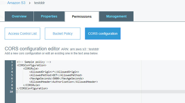
The following code must be entered into the setup:
You can read more about this setting here and set softer / tighter parameters. Initially, I thought that I needed to specify more methods (and not just GET), but it all works.
And now went the nuances.
When creating you need to specify the name, and then you need to be careful. Initially, I used a name containing hyphens, but could not connect to the cloud. It turned out that some individual characters actually cause this problem. There are workarounds, but they do not work for everyone. As a result, I began to use the variant of the name with underscore (digit_draw_recognize), there were no problems with it.
Next you need to specify the region. You can choose almost any, but it should be guided by this tablet .
First, we need Endpoint for the selected region, and secondly, it is easier to use regions that support versions 2 and 4 of the signature, so that you can use what is convenient. I chose US East (N. Virginia).
The remaining parameters when creating a bucket can not be changed.
Another important point is to configure CORS.
The following code must be entered into the setup:
<CORSConfiguration> <CORSRule> <AllowedOrigin>*</AllowedOrigin> <AllowedMethod>GET</AllowedMethod> <MaxAgeSeconds>3000</MaxAgeSeconds> <AllowedHeader>Authorization</AllowedHeader> </CORSRule> </CORSConfiguration> You can read more about this setting here and set softer / tighter parameters. Initially, I thought that I needed to specify more methods (and not just GET), but it all works.
Now actually about the code. For now, it’s about how to save files on Amazon. About receiving data from the cloud will be discussed later.
REGION_HOST = 's3-external-1.amazonaws.com' conn = S3Connection(os.environ['AWS_ACCESS_KEY_ID'], os.environ['AWS_SECRET_ACCESS_KEY'], host=REGION_HOST) bucket = conn.get_bucket('testddr') k = Key(bucket) fn = 'tmp/' + filename k.key = filename k.set_contents_from_filename(fn) The first step is to create a connection to the cloud. To do this, you must specify the Access Key ID, Secret Access Key and Region Host. We have already generated the keys, but it is dangerous to indicate them explicitly. This can be done only when testing the code locally. I hit the code on github a couple of times with openly specified keys - they were stolen for a couple of minutes. Do not repeat my mistakes. Heroku provides the ability to store keys and refer to them by name - more on this below. The region host is the endpoint value from the region label.
After that, you need to connect to the bucket - here it is already quite possible to specify the name directly.
Key used to work with objects in the basket. To save an object, you must specify the file name (k.key), and then call k.set_contents_from_filename() with the path to the file you want to save.Heroku
It's time to talk about how to place a website on Heroku. Heroku is a multi-language cloud platform that allows you to quickly and conveniently deploy web applications. It is possible to use Postgres and a lot of interesting things. Generally speaking, I could store images using Heroku resources, but I need to store different types of data, so it was easier to use a separate cloud.
Heroku offers several price plans, but for my application (including the full-fledged one, not this small one), the free one is enough. The only minus is that the application “falls asleep” after half an hour of activity and at the next launch it can spend 30 seconds to “wake up”.
You can find a lot of guides on deploying applications on Heroku (here is a link to the official one ), but most of them use the console, and I prefer to use interfaces. Besides, it seems to me much easier and more convenient.
Placing an application on Heroku
So to the point. To prepare the application, you need to create several files:
Now you can begin the process of creating an application. At this point there should be an account for heroku and a prepared github repository.
From the page with the list of applications, a new one is created:

Specify the name and country:

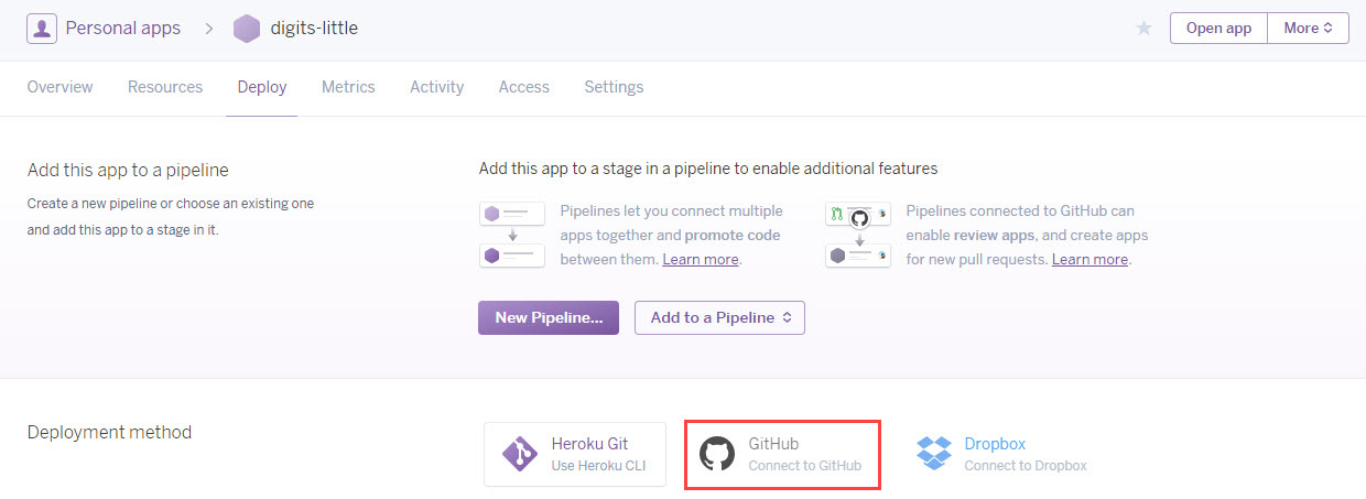
On the Deploy tab, select the connection to Github:
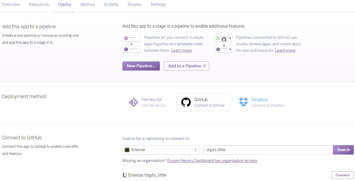
Connect and select the repository:
It makes sense to enable automatic updating of the application on Heroku every time you update the repository. And you can begin the deployment:
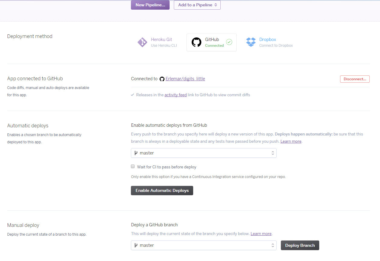
We look at the logs and hope that everything went well:

But still not everything is ready, before the first launch of the application on the settings tab, you need to set variables - keys for the Amazon cloud.

- Requires version control system .git. Usually it is created automatically when you create a github repository, but you need to check that it really is;
runtime.txt- this file should indicate the required version of the programming language used, in my case python-3.6.1;Procfileis a file with no extension. It indicates which commands should be run on heroku. This defines the type ofwebprocess that runs (my script) and the address:
web: python main.py runserver 0.0.0.0:5000 requirements.txt- a list of libraries that will be installed on Heroku. It is better to specify the necessary versions;- And the last thing - at least one file must be in the “tmp” folder, otherwise there may be problems with saving the files in this folder while the application is running;
Now you can begin the process of creating an application. At this point there should be an account for heroku and a prepared github repository.
From the page with the list of applications, a new one is created:
Specify the name and country:
On the Deploy tab, select the connection to Github:
Connect and select the repository:
It makes sense to enable automatic updating of the application on Heroku every time you update the repository. And you can begin the deployment:
We look at the logs and hope that everything went well:
But still not everything is ready, before the first launch of the application on the settings tab, you need to set variables - keys for the Amazon cloud.
Now you can run the application and work with it. This completes the site description for data collection. The following discussion focuses on data processing and the next stages of the project.
Image processing for models
I save the drawn images as pictures in the original format, so that you can always look at them and try different processing options.
Here are some examples:
The idea of image processing for my project is as follows (similar to mnist): the drawn figure is scaled to fit in a 20x20 square, keeping the proportions, and then placed in the center of a white square 28x28 in size. The following steps are necessary for this:
- find the borders of the image (the border has the shape of a rectangle);
- find the height and width of the bounded rectangle;
- to equate the larger side to 20, and the smaller to scale so as to keep the proportions;
- find the starting point for drawing the scaled digit on a 28x28 square and draw it;
- convert to np.array so that you can work with data and normalize;
Image processing
# img = Image.open('tmp/' + filename) # bbox = Image.eval(img, lambda px: 255-px).getbbox() if bbox == None: return None # widthlen = bbox[2] - bbox[0] heightlen = bbox[3] - bbox[1] # if heightlen > widthlen: widthlen = int(20.0 * widthlen / heightlen) heightlen = 20 else: heightlen = int(20.0 * widthlen / heightlen) widthlen = 20 # hstart = int((28 - heightlen) / 2) wstart = int((28 - widthlen) / 2) # img_temp = img.crop(bbox).resize((widthlen, heightlen), Image.NEAREST) # new_img = Image.new('L', (28,28), 255) new_img.paste(img_temp, (wstart, hstart)) # np.array imgdata = list(new_img.getdata()) img_array = np.array([(255.0 - x) / 255.0 for x in imgdata]) Image augmentation
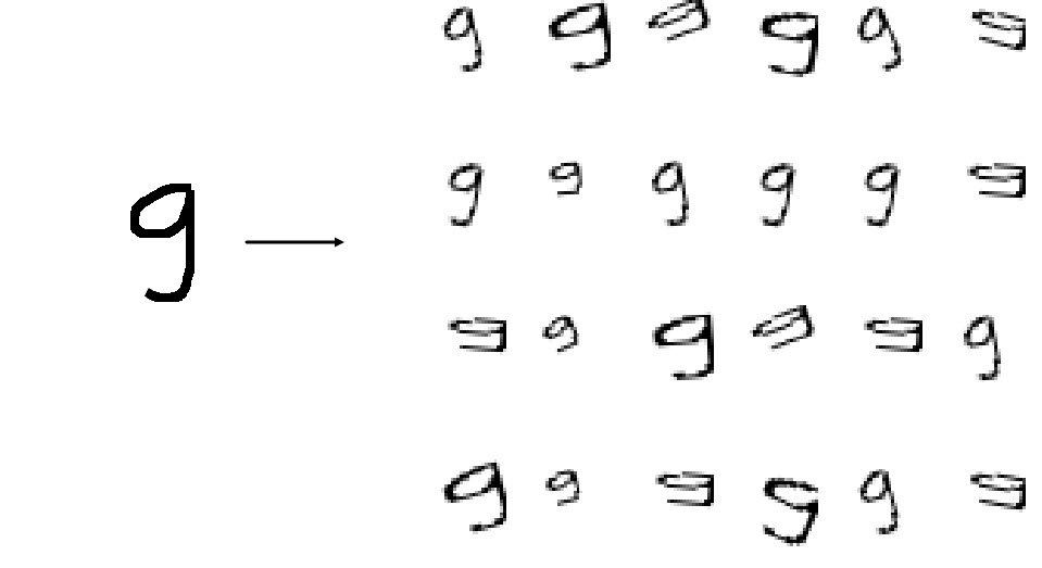
It is obvious that 1000 images are not enough for training the neural network, and in fact some of them need to be used for model validation. — , . , , . .
, . 2020 . 4 — 4 .
. , — 30 ; 5 , 12 . , 12 6.
# image = Image.open('tmp/' + filename) # ims_add = [] labs_add = [] # , angles = np.arange(-30, 30, 5) # bbox = Image.eval(image, lambda px: 255-px).getbbox() # widthlen = bbox[2] - bbox[0] heightlen = bbox[3] - bbox[1] # if heightlen > widthlen: widthlen = int(20.0 * widthlen/heightlen) heightlen = 20 else: heightlen = int(20.0 * widthlen/heightlen) widthlen = 20 # hstart = int((28 - heightlen) / 2) wstart = int((28 - widthlen) / 2) # 4 for i in [min(widthlen, heightlen), max(widthlen, heightlen)]: for j in [min(widthlen, heightlen), max(widthlen, heightlen)]: # resized_img = image.crop(bbox).resize((i, j), Image.NEAREST) # resized_image = Image.new('L', (28,28), 255) resized_image.paste(resized_img, (wstart, hstart)) # 6 12. angles_ = random.sample(set(angles), 6) for angle in angles_: # transformed_image = transform.rotate(np.array(resized_image), angle, cval=255, preserve_range=True).astype(np.uint8) labs_add.append(int(label)) # img_temp = Image.fromarray(np.uint8(transformed_image)) # np.array imgdata = list(img_temp.getdata()) normalized_img = [(255.0 - x) / 255.0 for x in imgdata] ims_add.append(normalized_img) :
800 * 24 = 19200 200 . .
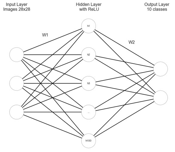
FNN
feed forward neural net. , cs231n, .
import matplotlib.pyplot as plt #https://gist.github.com/anbrjohn/7116fa0b59248375cd0c0371d6107a59 def draw_neural_net(ax, left, right, bottom, top, layer_sizes, layer_text=None): ''' :parameters: - ax : matplotlib.axes.AxesSubplot The axes on which to plot the cartoon (get eg by plt.gca()) - left : float The center of the leftmost node(s) will be placed here - right : float The center of the rightmost node(s) will be placed here - bottom : float The center of the bottommost node(s) will be placed here - top : float The center of the topmost node(s) will be placed here - layer_sizes : list of int List of layer sizes, including input and output dimensionality - layer_text : list of str List of node annotations in top-down left-right order ''' n_layers = len(layer_sizes) v_spacing = (top - bottom)/float(max(layer_sizes)) h_spacing = (right - left)/float(len(layer_sizes) - 1) ax.axis('off') # Nodes for n, layer_size in enumerate(layer_sizes): layer_top = v_spacing*(layer_size - 1)/2. + (top + bottom)/2. for m in range(layer_size): x = n*h_spacing + left y = layer_top - m*v_spacing circle = plt.Circle((x,y), v_spacing/4., color='w', ec='k', zorder=4) ax.add_artist(circle) # Node annotations if layer_text: text = layer_text.pop(0) plt.annotate(text, xy=(x, y), zorder=5, ha='center', va='center') # Edges for n, (layer_size_a, layer_size_b) in enumerate(zip(layer_sizes[:-1], layer_sizes[1:])): layer_top_a = v_spacing*(layer_size_a - 1)/2. + (top + bottom)/2. layer_top_b = v_spacing*(layer_size_b - 1)/2. + (top + bottom)/2. for m in range(layer_size_a): for o in range(layer_size_b): line = plt.Line2D([n*h_spacing + left, (n + 1)*h_spacing + left], [layer_top_a - m*v_spacing, layer_top_b - o*v_spacing], c='k') ax.add_artist(line) node_text = ['','','','h1','h2','h3','...', 'h100'] fig = plt.figure(figsize=(8, 8)) ax = fig.gca() draw_neural_net(ax, .1, .9, .1, .9, [3, 5, 2], node_text) plt.text(0.1, 0.95, "Input Layer\nImages 28x28", ha='center', va='top', fontsize=16) plt.text(0.26, 0.78, "W1", ha='center', va='top', fontsize=16) plt.text(0.5, 0.95, "Hidden Layer\n with ReLU", ha='center', va='top', fontsize=16) plt.text(0.74, 0.74, "W2", ha='center', va='top', fontsize=16) plt.text(0.88, 0.95, "Output Layer\n10 classes", ha='center', va='top', fontsize=16) plt.show() FNN
import numpy as np class TwoLayerNet(object): """ A two-layer fully-connected neural network. The net has an input dimension of N, a hidden layer dimension of H, and performs classification over C classes. We train the network with a softmax loss function and L2 regularization on the weight matrices. The network uses a ReLU nonlinearity after the first fully connected layer. In other words, the network has the following architecture: input - fully connected layer - ReLU - fully connected layer - softmax The outputs of the second fully-connected layer are the scores for each class. """ def __init__(self, input_size, hidden_size, output_size, std): """ Initialize the model. Weights are initialized following Xavier intialization and biases are initialized to zero. Weights and biases are stored in the variable self.params, which is a dictionary with the following keys: W1: First layer weights; has shape (D, H) b1: First layer biases; has shape (H,) W2: Second layer weights; has shape (H, C) b2: Second layer biases; has shape (C,) Inputs: - input_size: The dimension D of the input data. - hidden_size: The number of neurons H in the hidden layer. - output_size: The number of classes C. """ self.params = {} self.params['W1'] = (((2 / input_size) ** 0.5) * np.random.randn(input_size, hidden_size)) self.params['b1'] = np.zeros(hidden_size) self.params['W2'] = (((2 / hidden_size) ** 0.5) * np.random.randn(hidden_size, output_size)) self.params['b2'] = np.zeros(output_size) def loss(self, X, y=None, reg=0.0): """ Compute the loss and gradients for a two layer fully connected neural network. Inputs: - X: Input data of shape (N, D). X[i] is a training sample. - y: Vector of training labels. y[i] is the label for X[i], and each y[i] is an integer in the range 0 <= y[i] < C. - reg: Regularization strength. Returns: - loss: Loss (data loss and regularization loss) for this batch of training samples. - grads: Dictionary mapping parameter names to gradients of those parameters with respect to the loss function; has the same keys as self.params. """ # Unpack variables from the params dictionary W1, b1 = self.params['W1'], self.params['b1'] W2, b2 = self.params['W2'], self.params['b2'] N, D = X.shape # Compute the forward pass l1 = X.dot(W1) + b1 l1[l1 < 0] = 0 l2 = l1.dot(W2) + b2 exp_scores = np.exp(l2) probs = exp_scores / np.sum(exp_scores, axis=1, keepdims=True) scores = l2 # Compute the loss W1_r = 0.5 * reg * np.sum(W1 * W1) W2_r = 0.5 * reg * np.sum(W2 * W2) loss = -np.sum(np.log(probs[range(y.shape[0]), y]))/N + W1_r + W2_r # Backward pass: compute gradients grads = {} probs[range(X.shape[0]),y] -= 1 dW2 = np.dot(l1.T, probs) dW2 /= X.shape[0] dW2 += reg * W2 grads['W2'] = dW2 grads['b2'] = np.sum(probs, axis=0, keepdims=True) / X.shape[0] delta = probs.dot(W2.T) delta = delta * (l1 > 0) grads['W1'] = np.dot(XT, delta)/ X.shape[0] + reg * W1 grads['b1'] = np.sum(delta, axis=0, keepdims=True) / X.shape[0] return loss, grads def train(self, X, y, X_val, y_val, learning_rate=1e-3, learning_rate_decay=0.95, reg=5e-6, num_iters=100, batch_size=24, verbose=False): """ Train this neural network using stochastic gradient descent. Inputs: - X: A numpy array of shape (N, D) giving training data. - y: A numpy array f shape (N,) giving training labels; y[i] = c means that [i] has label c, where 0 <= c < C. - X_val: A numpy array of shape (N_val, D); validation data. - y_val: A numpy array of shape (N_val,); validation labels. - learning_rate: Scalar giving learning rate for optimization. - learning_rate_decay: Scalar giving factor used to decay the learning rate each epoch. - reg: Scalar giving regularization strength. - num_iters: Number of steps to take when optimizing. - batch_size: Number of training examples to use per step. - verbose: boolean; if true print progress during optimization. """ num_train = X.shape[0] iterations_per_epoch = max(num_train / batch_size, 1) # Use SGD to optimize the parameters in self.model loss_history = [] train_acc_history = [] val_acc_history = [] # Training cycle for it in range(num_iters): # Mini-batch selection indexes = np.random.choice(X.shape[0], batch_size, replace=True) X_batch = X[indexes] y_batch = y[indexes] # Compute loss and gradients using the current minibatch loss, grads = self.loss(X_batch, y=y_batch, reg=reg) loss_history.append(loss) # Update weights self.params['W1'] -= learning_rate * grads['W1'] self.params['b1'] -= learning_rate * grads['b1'][0] self.params['W2'] -= learning_rate * grads['W2'] self.params['b2'] -= learning_rate * grads['b2'][0] if verbose and it % 100 == 0: print('iteration %d / %d: loss %f' % (it, num_iters, loss)) # Every epoch, check accuracy and decay learning rate. if it % iterations_per_epoch == 0: # Check accuracy train_acc = (self.predict(X_batch)==y_batch).mean() val_acc = (self.predict(X_val) == y_val).mean() train_acc_history.append(train_acc) val_acc_history.append(val_acc) # Decay learning rate learning_rate *= learning_rate_decay return { 'loss_history': loss_history, 'train_acc_history': train_acc_history, 'val_acc_history': val_acc_history, } def predict(self, X): """ Use the trained weights of this two-layer network to predict labels for points. For each data point we predict scores for each of the C classes, and assign each data point to the class with the highest score. Inputs: - X: A numpy array of shape (N, D) giving N D-dimensional data points to classify. Returns: - y_pred: A numpy array of shape (N,) giving predicted labels for each of elements of X. For all i, y_pred[i] = c means that X[i] is predicted to have class c, where 0 <= c < C. """ l1 = X.dot(self.params['W1']) + self.params['b1'] l1[l1 < 0] = 0 l2 = l1.dot(self.params['W2']) + self.params['b2'] exp_scores = np.exp(l2) probs = exp_scores / np.sum(exp_scores, axis=1, keepdims=True) y_pred = np.argmax(probs, axis=1) return y_pred def predict_single(self, X): """ Use the trained weights of this two-layer network to predict label for data point. We predict scores for each of the C classes, and assign the data point to the class with the highest score. Inputs: - X: A numpy array of shape (N, D) giving N D-dimensional data points to classify. Returns: - y_pred: A numpy array of shape (1,) giving predicted labels for X. """ l1 = X.dot(self.params['W1']) + self.params['b1'] l1[l1 < 0] = 0 l2 = l1.dot(self.params['W2']) + self.params['b2'] exp_scores = np.exp(l2) y_pred = np.argmax(exp_scores) return y_pred FNN

:
- (Xavier). 2 / . ;
- loss L2 ;
- train -. . , learning rate decay;
- predict_single , predict — ;
:
input_size = 28 * 28 hidden_size = 100 num_classes = 10 net = tln(input_size, hidden_size, num_classes) :
- ;
- -, ;
- learning rate decay, learning rate ;
- ;
- verbose / ;
stats = net.train(X_train_, y_train_, X_val, y_val, num_iters=19200, batch_size=24, learning_rate=0.1, learning_rate_decay=0.95, reg=0.001, verbose=True) , loss , :
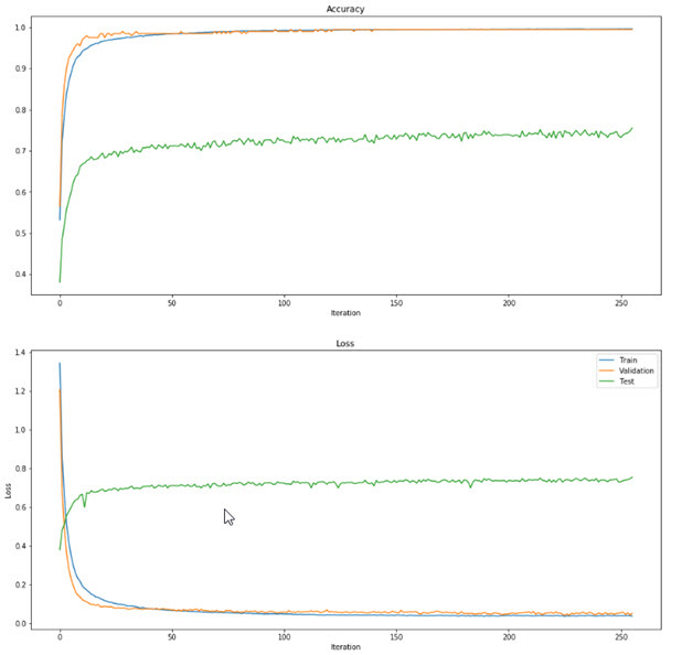
plt.subplot(2, 1, 1) plt.plot(stats['loss_history']) plt.title('Loss history') plt.xlabel('Iteration') plt.ylabel('Loss') plt.subplot(2, 1, 2) plt.plot(stats['train_acc_history'], label='train') plt.plot(stats['val_acc_history'], label='val') plt.title('Classification accuracy history') plt.xlabel('Epoch') plt.ylabel('Clasification accuracy') plt.legend() plt.show() — . , , — , . . , , . , , , .
, . . learning rate, regularization, , -; , . .
Selection of parameters
from itertools import product best_net = None results = {} best_val = -1 learning_rates = [0.001, 0.1, 0.01, 0.5] regularization_strengths = [0.001, 0.1, 0.01] hidden_size = [5, 10, 20] epochs = [1000, 1500, 2000] batch_sizes = [24, 12] best_params = 0 best_params = 0 for v in product(learning_rates, regularization_strengths, hidden_size, epochs, batch_sizes): print('learning rate: {0}, regularization strength: {1}, hidden size: {2}, \ iterations: {3}, batch_size: {4}.'.format(v[0], v[1], v[2], v[3], v[4])) net = TwoLayerNet(input_size, v[2], num_classes) stats = net.train(X_train_, y_train, X_val_, y_val, num_iters=v[3], batch_size=v[4], learning_rate=v[0], learning_rate_decay=0.95, reg=v[1], verbose=False) y_train_pred = net.predict(X_train_) train_acc = np.mean(y_train == y_train_pred) val_acc = (net.predict(X_val_) == y_val).mean() print('Validation accuracy: ', val_acc) results[(v[0], v[1], v[2], v[3], v[4])] = val_acc if val_acc > best_val: best_val = val_acc best_net = net best_params = (v[0], v[1], v[2], v[3], v[4]) , , , - . , , learning rate . . - , : , 1 . 1 24 , - . 24.
MNIST, MNIST.
MNIST
def read(path = "."): fname_img = os.path.join(path, 't10k-images.idx3-ubyte') fname_lbl = os.path.join(path, 't10k-labels.idx1-ubyte') with open(fname_lbl, 'rb') as flbl: magic, num = struct.unpack(">II", flbl.read(8)) lbl = np.fromfile(flbl, dtype=np.int8) with open(fname_img, 'rb') as fimg: magic, num, rows, cols = struct.unpack(">IIII", fimg.read(16)) img = np.fromfile(fimg, dtype=np.uint8).reshape(len(lbl), rows, cols) get_img = lambda idx: (lbl[idx], img[idx]) for i in range(len(lbl)): yield get_img(i) test = list(read(path="/MNIST_data")) mnist_labels = np.array([i[0] for i in test]).astype(int) mnist_picts = np.array([i[1] for i in test]).reshape(10000, 784) / 255 y_mnist = np.array(mnist_labels).astype(int) :
, ~10 , .
, , MNIST . , , MNIST . CNN Tensorflow MNIST . MNIST 99%+ ( ), : 78.5% 63.35% . , MNIST , MNIST.
, :
- ;
- /;
- : , , rmsprop;
. , .
:
net.param , — , — . numpy : np.save('tmp/updated_weights.npy', net.params) . np.load('models/original_weights.npy')[()] ( [()] , )..
FNN
. :
- , . ;
- , ;
- (1 , 24);
- (learning rate ) ;
- predict-single 3 . , ;
FNN
import numpy as np class FNN(object): """ A two-layer fully-connected neural network. The net has an input dimension of N, a hidden layer dimension of H, and performs classification over C classes. We train the network with a softmax loss function and L2 regularization on the weight matrices. The network uses a ReLU nonlinearity after the first fully connected layer. In other words, the network has the following architecture: input - fully connected layer - ReLU - fully connected layer - softmax The outputs of the second fully-connected layer are the scores for each class. """ def __init__(self, weights,input_size=28*28,hidden_size=100,output_size=10): """ Initialize the model. Weights are initialized following Xavier intialization and biases are initialized to zero. Weights and biases are stored in the variable self.params, which is a dictionary with the following keys: W1: First layer weights; has shape (D, H) b1: First layer biases; has shape (H,) W2: Second layer weights; has shape (H, C) b2: Second layer biases; has shape (C,) Inputs: - input_size: The dimension D of the input data. - hidden_size: The number of neurons H in the hidden layer. - output_size: The number of classes C. """ self.params = {} self.params['W1'] = weights['W1'] self.params['b1'] = weights['b1'] self.params['W2'] = weights['W2'] self.params['b2'] = weights['b2'] def loss(self, X, y, reg=0.0): """ Compute the loss and gradients for a two layer fully connected neural network. Inputs: - X: Input data of shape (N, D). X[i] is a training sample. - y: Vector of training labels. y[i] is the label for X[i], and each y[i] is an integer in the range 0 <= y[i] < C. - reg: Regularization strength. Returns: - loss: Loss (data loss and regularization loss) for this batch of training samples. - grads: Dictionary mapping parameter names to gradients of those parameters with respect to the loss function; has the same keys as self.params. """ # Unpack variables from the params dictionary W1, b1 = self.params['W1'], self.params['b1'] W2, b2 = self.params['W2'], self.params['b2'] N, D = X.shape # Compute the forward pass l1 = X.dot(W1) + b1 l1[l1 < 0] = 0 l2 = l1.dot(W2) + b2 exp_scores = np.exp(l2) probs = exp_scores / np.sum(exp_scores, axis=1, keepdims=True) # Backward pass: compute gradients grads = {} probs[range(X.shape[0]), y] -= 1 dW2 = np.dot(l1.T, probs) dW2 /= X.shape[0] dW2 += reg * W2 grads['W2'] = dW2 grads['b2'] = np.sum(probs, axis=0, keepdims=True) / X.shape[0] delta = probs.dot(W2.T) delta = delta * (l1 > 0) grads['W1'] = np.dot(XT, delta)/ X.shape[0] + reg * W1 grads['b1'] = np.sum(delta, axis=0, keepdims=True) / X.shape[0] return grads def train(self, X, y, learning_rate=0.1*(0.95**24)/32, reg=0.001, batch_size=24): """ Train this neural network using stochastic gradient descent. Inputs: - X: A numpy array of shape (N, D) giving training data. - y: A numpy array f shape (N,) giving training labels; y[i] = c means that [i] has label c, where 0 <= c < C. - X_val: A numpy array of shape (N_val, D); validation data. - y_val: A numpy array of shape (N_val,); validation labels. - learning_rate: Scalar giving learning rate for optimization. - learning_rate_decay: Scalar giving factor used to decay the learning rate each epoch. - reg: Scalar giving regularization strength. - num_iters: Number of steps to take when optimizing. - batch_size: Number of training examples to use per step. - verbose: boolean; if true print progress during optimization. """ num_train = X.shape[0] # Compute loss and gradients using the current minibatch grads = self.loss(X, y, reg=reg) self.params['W1'] -= learning_rate * grads['W1'] self.params['b1'] -= learning_rate * grads['b1'][0] self.params['W2'] -= learning_rate * grads['W2'] self.params['b2'] -= learning_rate * grads['b2'][0] def predict(self, X): """ Use the trained weights of this two-layer network to predict labels for points. For each data point we predict scores for each of the C classes, and assign each data point to the class with the highest score. Inputs: - X: A numpy array of shape (N, D) giving N D-dimensional data points to classify. Returns: - y_pred: A numpy array of shape (N,) giving predicted labels for each of elements of X. For all i, y_pred[i] = c means that X[i] is predicted to have class c, where 0 <= c < C. """ l1 = X.dot(self.params['W1']) + self.params['b1'] l1[l1 < 0] = 0 l2 = l1.dot(self.params['W2']) + self.params['b2'] exp_scores = np.exp(l2) probs = exp_scores / np.sum(exp_scores, axis=1, keepdims=True) y_pred = np.argmax(probs, axis=1) return y_pred def predict_single(self, X): """ Use the trained weights of this two-layer network to predict label for data point. We predict scores for each of the C classes, and assign the data point to the class with the highest score. Inputs: - X: A numpy array of shape (N, D) giving N D-dimensional data points to classify. Returns: - top_3: a list of 3 top most probable predictions with their probabilities as tuples. """ l1 = X.dot(self.params['W1']) + self.params['b1'] l1[l1 < 0] = 0 l2 = l1.dot(self.params['W2']) + self.params['b2'] exp_scores = np.exp(l2) probs = exp_scores / np.sum(exp_scores) y_pred = np.argmax(exp_scores) top_3 = list(zip(np.argsort(probs)[::-1][:3], np.round(probs[np.argsort(probs)[::-1][:3]] * 100, 2))) return top_3 , — , learning rate.
learning rate . 0.1, 24 0.1 x (0.95 ^ 24). , — 800 . , . 0.1 x (0.95 ^ 24) / 32. , .
CNN
, FNN , CNN, , CNN, .
CNN cs231n Tenforlow MNIST, .
import os import numpy as np import matplotlib.pyplot as plt plt.rcdefaults() from matplotlib.lines import Line2D from matplotlib.patches import Rectangle from matplotlib.collections import PatchCollection #https://github.com/gwding/draw_convnet NumConvMax = 8 NumFcMax = 20 White = 1. Light = 0.7 Medium = 0.5 Dark = 0.3 Black = 0. def add_layer(patches, colors, size=24, num=5, top_left=[0, 0], loc_diff=[3, -3], ): # add a rectangle top_left = np.array(top_left) loc_diff = np.array(loc_diff) loc_start = top_left - np.array([0, size]) for ind in range(num): patches.append(Rectangle(loc_start + ind * loc_diff, size, size)) if ind % 2: colors.append(Medium) else: colors.append(Light) def add_mapping(patches, colors, start_ratio, patch_size, ind_bgn, top_left_list, loc_diff_list, num_show_list, size_list): start_loc = top_left_list[ind_bgn] \ + (num_show_list[ind_bgn] - 1) * np.array(loc_diff_list[ind_bgn]) \ + np.array([start_ratio[0] * size_list[ind_bgn], -start_ratio[1] * size_list[ind_bgn]]) end_loc = top_left_list[ind_bgn + 1] \ + (num_show_list[ind_bgn + 1] - 1) \ * np.array(loc_diff_list[ind_bgn + 1]) \ + np.array([(start_ratio[0] + .5 * patch_size / size_list[ind_bgn]) * size_list[ind_bgn + 1], -(start_ratio[1] - .5 * patch_size / size_list[ind_bgn]) * size_list[ind_bgn + 1]]) patches.append(Rectangle(start_loc, patch_size, patch_size)) colors.append(Dark) patches.append(Line2D([start_loc[0], end_loc[0]], [start_loc[1], end_loc[1]])) colors.append(Black) patches.append(Line2D([start_loc[0] + patch_size, end_loc[0]], [start_loc[1], end_loc[1]])) colors.append(Black) patches.append(Line2D([start_loc[0], end_loc[0]], [start_loc[1] + patch_size, end_loc[1]])) colors.append(Black) patches.append(Line2D([start_loc[0] + patch_size, end_loc[0]], [start_loc[1] + patch_size, end_loc[1]])) colors.append(Black) def label(xy, text, xy_off=[0, 4]): plt.text(xy[0] + xy_off[0], xy[1] + xy_off[1], text, family='sans-serif', size=8) if __name__ == '__main__': fc_unit_size = 2 layer_width = 40 patches = [] colors = [] fig, ax = plt.subplots() ############################ # conv layers size_list = [28, 28, 14, 14, 7] num_list = [1, 16, 16, 32, 32] x_diff_list = [0, layer_width, layer_width, layer_width, layer_width] text_list = ['Inputs'] + ['Feature\nmaps'] * (len(size_list) - 1) loc_diff_list = [[3, -3]] * len(size_list) num_show_list = list(map(min, num_list, [NumConvMax] * len(num_list))) top_left_list = np.c_[np.cumsum(x_diff_list), np.zeros(len(x_diff_list))] for ind in range(len(size_list)): add_layer(patches, colors, size=size_list[ind], num=num_show_list[ind], top_left=top_left_list[ind], loc_diff=loc_diff_list[ind]) label(top_left_list[ind], text_list[ind] + '\n{}@{}x{}'.format( num_list[ind], size_list[ind], size_list[ind])) ############################ # in between layers start_ratio_list = [[0.4, 0.5], [0.4, 0.8], [0.4, 0.5], [0.4, 0.8]] patch_size_list = [4, 2, 4, 2] ind_bgn_list = range(len(patch_size_list)) text_list = ['Convolution', 'Max-pooling', 'Convolution', 'Max-pooling'] for ind in range(len(patch_size_list)): add_mapping(patches, colors, start_ratio_list[ind], patch_size_list[ind], ind, top_left_list, loc_diff_list, num_show_list, size_list) label(top_left_list[ind], text_list[ind] + '\n{}x{} kernel'.format( patch_size_list[ind], patch_size_list[ind]), xy_off=[26, -65]) ############################ # fully connected layers size_list = [fc_unit_size, fc_unit_size, fc_unit_size] num_list = [1568, 625, 10] num_show_list = list(map(min, num_list, [NumFcMax] * len(num_list))) x_diff_list = [sum(x_diff_list) + layer_width, layer_width, layer_width] top_left_list = np.c_[np.cumsum(x_diff_list), np.zeros(len(x_diff_list))] loc_diff_list = [[fc_unit_size, -fc_unit_size]] * len(top_left_list) text_list = ['Hidden\nunits'] * (len(size_list) - 1) + ['Outputs'] for ind in range(len(size_list)): add_layer(patches, colors, size=size_list[ind], num=num_show_list[ind], top_left=top_left_list[ind], loc_diff=loc_diff_list[ind]) label(top_left_list[ind], text_list[ind] + '\n{}'.format( num_list[ind])) text_list = ['Flatten\n', 'Fully\nconnected', 'Fully\nconnected'] for ind in range(len(size_list)): label(top_left_list[ind], text_list[ind], xy_off=[-10, -65]) ############################ colors += [0, 1] collection = PatchCollection(patches, cmap=plt.cm.gray) collection.set_array(np.array(colors)) ax.add_collection(collection) plt.tight_layout() plt.axis('equal') plt.axis('off') plt.show() fig.set_size_inches(8, 2.5) fig_dir = './' fig_ext = '.png' fig.savefig(os.path.join(fig_dir, 'convnet_fig' + fig_ext), bbox_inches='tight', pad_inches=0) Tensorflow, , FNN numpy.
CNN
import tensorflow as tf # Define architecture def model(X, w, w3, w4, w_o, p_keep_conv, p_keep_hidden): l1a = tf.nn.relu( tf.nn.conv2d( X, w, strides=[1, 1, 1, 1], padding='SAME' ) + b1 ) l1 = tf.nn.max_pool( l1a, ksize=[1, 2, 2, 1], strides=[1, 2, 2, 1], padding='SAME' ) l1 = tf.nn.dropout(l1, p_keep_conv) l3a = tf.nn.relu( tf.nn.conv2d( l1, w3, strides=[1, 1, 1, 1], padding='SAME' ) + b3 ) l3 = tf.nn.max_pool( l3a, ksize=[1, 2, 2, 1], strides=[1, 2, 2, 1], padding='SAME' ) # Reshaping for dense layer l3 = tf.reshape(l3, [-1, w4.get_shape().as_list()[0]]) l3 = tf.nn.dropout(l3, p_keep_conv) l4 = tf.nn.relu(tf.matmul(l3, w4) + b4) l4 = tf.nn.dropout(l4, p_keep_hidden) pyx = tf.matmul(l4, w_o) + b5 return pyx tf.reset_default_graph() # Define variables init_op = tf.global_variables_initializer() X = tf.placeholder("float", [None, 28, 28, 1]) Y = tf.placeholder("float", [None, 10]) w = tf.get_variable("w", shape=[4, 4, 1, 16], initializer=tf.contrib.layers.xavier_initializer()) b1 = tf.get_variable(name="b1", shape=[16], initializer=tf.zeros_initializer()) w3 = tf.get_variable("w3", shape=[4, 4, 16, 32], initializer=tf.contrib.layers.xavier_initializer()) b3 = tf.get_variable(name="b3", shape=[32], initializer=tf.zeros_initializer()) w4 = tf.get_variable("w4", shape=[32 * 7 * 7, 625], initializer=tf.contrib.layers.xavier_initializer()) b4 = tf.get_variable(name="b4", shape=[625], initializer=tf.zeros_initializer()) w_o = tf.get_variable("w_o", shape=[625, 10], initializer=tf.contrib.layers.xavier_initializer()) b5 = tf.get_variable(name="b5", shape=[10], initializer=tf.zeros_initializer()) # Dropout rate p_keep_conv = tf.placeholder("float") p_keep_hidden = tf.placeholder("float") py_x = model(X, w, w3, w4, w_o, p_keep_conv, p_keep_hidden) reg_losses = tf.get_collection(tf.GraphKeys.REGULARIZATION_LOSSES) reg_constant = 0.01 cost = tf.reduce_mean(tf.nn.softmax_cross_entropy_with_logits(logits=py_x, labels=Y) + reg_constant * sum(reg_losses)) train_op = tf.train.RMSPropOptimizer(0.0001, 0.9).minimize(cost) predict_op = tf.argmax(py_x, 1) #Training train_acc = [] val_acc = [] test_acc = [] train_loss = [] val_loss = [] test_loss = [] with tf.Session() as sess: tf.global_variables_initializer().run() # Training iterations for i in range(256): # Mini-batch training_batch = zip(range(0, len(trX), batch_size), range(batch_size, len(trX)+1, batch_size)) for start, end in training_batch: sess.run(train_op, feed_dict={X: trX[start:end], Y: trY[start:end], p_keep_conv: 0.8, p_keep_hidden: 0.5}) # Comparing labels with predicted values train_acc = np.mean(np.argmax(trY, axis=1) == sess.run(predict_op, feed_dict={X: trX, Y: trY, p_keep_conv: 1.0, p_keep_hidden: 1.0})) train_acc.append(train_acc) val_acc = np.mean(np.argmax(teY, axis=1) == sess.run(predict_op, feed_dict={X: teX, Y: teY, p_keep_conv: 1.0, p_keep_hidden: 1.0})) val_acc.append(val_acc) test_acc = np.mean(np.argmax(mnist.test.labels, axis=1) == sess.run(predict_op, feed_dict={X: mnist_test_images, Y: mnist.test.labels, p_keep_conv: 1.0, p_keep_hidden: 1.0})) test_acc.append(test_acc) print('Step {0}. Train accuracy: {3}. Validation accuracy: {1}. \ Test accuracy: {2}.'.format(i, val_acc, test_acc, train_acc)) _, loss_train = sess.run([predict_op, cost], feed_dict={X: trX, Y: trY, p_keep_conv: 1.0, p_keep_hidden: 1.0}) train_loss.append(loss_train) _, loss_val = sess.run([predict_op, cost], feed_dict={X: teX, Y: teY, p_keep_conv: 1.0, p_keep_hidden: 1.0}) val_loss.append(loss_val) _, loss_test = sess.run([predict_op, cost], feed_dict={X: mnist_test_images, Y: mnist.test.labels, p_keep_conv: 1.0, p_keep_hidden: 1.0}) test_loss.append(loss_test) print('Train loss: {0}. Validation loss: {1}. \ Test loss: {2}.'.format(loss_train, loss_val, loss_test)) # Saving model all_saver = tf.train.Saver() all_saver.save(sess, '/resources/data.chkp') #Predicting with tf.Session() as sess: # Restoring model saver = tf.train.Saver() saver.restore(sess, "./data.chkp") # Prediction pr = sess.run(predict_op, feed_dict={X: mnist_test_images, Y: mnist.test.labels, p_keep_conv: 1.0, p_keep_hidden: 1.0}) print(np.mean(np.argmax(mnist.test.labels, axis=1) == sess.run(predict_op, feed_dict={X: mnist_test_images, Y: mnist.test.labels, p_keep_conv: 1.0, p_keep_hidden: 1.0}))) CNN
CNN FNN , . CNN — , - .
. ( N x 28 x 28 x 1), «» ( ), . . . . : . , RGB. .

, , 1, . zero-padding, 0 , . :
max pooling ( , max ). , . : , . cs231n.
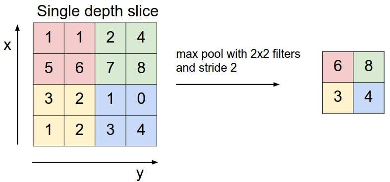
Max pooling ( 2 2) . . ; 2.
. . , , .
, .
N x 28 x 28 x 1. 4 4 16, zero-padding (
, . , «» .
. ( N x 28 x 28 x 1), «» ( ), . . . . : . , RGB. .
, , 1, . zero-padding, 0 , . :
- , , ;
- , ;
- , ;
- , , , zero-padding , ;
max pooling ( , max ). , . : , . cs231n.
Max pooling ( 2 2) . . ; 2.
. . , , .
, .
N x 28 x 28 x 1. 4 4 16, zero-padding (
padding='SAME' Tensorflow) , N x 28 x 28 x 16. max pooling 2 2 2, N x 14 x 14 x 16. 4 4 32 zero-padding, N x 14 x 14 x 32. max pooling ( ) N x 7 x 7 x 32. . 32 * 7 * 7 625 1568 625, N 625. 625 10 10 ., . , «» .
:
- , ;
- : ;
- X, y dropout ;
- Cost softmax_cross_entropy_with_logits L2;
- — RMSPropOptimizer;
- (256), ;
- dropout 0.2 convolutional 0.5 . , «» (MNIST) ;
- , /. , , , ;
MNIST TF :
from tensorflow.examples.tutorials.mnist import input_data mnist = input_data.read_data_sets('MNIST_data', one_hot=True) mnist_test_images = mnist.test.images.reshape(-1, 28, 28, 1) , FNN, - , :
trX = X_train.reshape(-1, 28, 28, 1) # 28x28x1 teX = X_val.reshape(-1, 28, 28, 1) enc = OneHotEncoder() enc.fit(y.reshape(-1, 1), 10).toarray() # 10x1 trY = enc.fit_transform(y_train.reshape(-1, 1)).toarray() teY = enc.fit_transform(y_val.reshape(-1, 1)).toarray() CNN FNN, -. - , CNN , . , :
:
, , ~100 .
CNN , FNN: , 1 , -3 .
CNN
import numpy as np import boto import boto3 from boto.s3.key import Key from boto.s3.connection import S3Connection import tensorflow as tf import os class CNN(object): """ Convolutional neural network with several levels. The architecture is the following: input - conv - relu - pool - dropout - conv - relu - pool - dropout - fully connected layer - dropout - fully connected layer The outputs of the second fully-connected layer are the scores for each class. """ def __init__(self): """ Initialize the model. Weights are passed into the class. """ self.params = {} def train(self, image, digit): """ Train this neural network. 1 step of gradient descent. Inputs: - X: A numpy array of shape (N, 784) giving training data. - y: A numpy array f shape (N,) giving training labels; y[i] = c means that X[i] has label c, where 0 <= c < C. """ tf.reset_default_graph() init_op = tf.global_variables_initializer() X = tf.placeholder("float", [None, 28, 28, 1]) Y = tf.placeholder("float", [None, 10]) w = tf.get_variable("w", shape=[4, 4, 1, 16], initializer=tf.contrib.layers.xavier_initializer()) b1 = tf.get_variable(name="b1", shape=[16], initializer=tf.zeros_initializer()) w3 = tf.get_variable("w3", shape=[4, 4, 16, 32], initializer=tf.contrib.layers.xavier_initializer()) b3 = tf.get_variable(name="b3", shape=[32], initializer=tf.zeros_initializer()) w4 = tf.get_variable("w4", shape=[32 * 7 * 7, 625], initializer=tf.contrib.layers.xavier_initializer()) b4 = tf.get_variable(name="b4", shape=[625], initializer=tf.zeros_initializer()) w_o = tf.get_variable("w_o", shape=[625, 10], initializer=tf.contrib.layers.xavier_initializer()) b5 = tf.get_variable(name="b5", shape=[10], initializer=tf.zeros_initializer()) p_keep_conv = tf.placeholder("float") p_keep_hidden = tf.placeholder("float") l1a = tf.nn.relu( tf.nn.conv2d( X, w, strides=[1, 1, 1, 1], padding='SAME' ) + b1 ) l1 = tf.nn.max_pool( l1a, ksize=[1, 2, 2, 1], strides=[1, 2, 2, 1], padding='SAME') l1 = tf.nn.dropout(l1, p_keep_conv) l3a = tf.nn.relu( tf.nn.conv2d( l1, w3, strides=[1, 1, 1, 1], padding='SAME' ) + b3 ) l3 = tf.nn.max_pool( l3a, ksize=[1, 2, 2, 1], strides=[1, 2, 2, 1], padding='SAME') #Reshape for matmul l3 = tf.reshape(l3, [-1, w4.get_shape().as_list()[0]]) l3 = tf.nn.dropout(l3, p_keep_conv) l4 = tf.nn.relu(tf.matmul(l3, w4) + b4) l4 = tf.nn.dropout(l4, p_keep_hidden) py_x = tf.matmul(l4, w_o) + b5 # Cost with L2 reg_losses = tf.get_collection(tf.GraphKeys.REGULARIZATION_LOSSES) reg_constant = 0.01 cost = tf.reduce_mean( tf.nn.softmax_cross_entropy_with_logits(logits=py_x, labels=Y) + reg_constant * sum(reg_losses) ) train_op = tf.train.RMSPropOptimizer(0.00001).minimize(cost) predict_op = tf.argmax(py_x, 1) with tf.Session() as sess: # Load weights saver = tf.train.Saver() saver.restore(sess, "./tmp/data-all_2_updated.chkp") trX = image.reshape(-1, 28, 28, 1) trY = np.eye(10)[digit] sess.run(train_op, feed_dict={X: trX, Y: trY, p_keep_conv: 1, p_keep_hidden: 1}) # Save updated weights all_saver = tf.train.Saver() all_saver.save(sess, './tmp/data-all_2_updated.chkp') def predict(self, image, weights='original'): """ Generate prediction for one or several digits. Weights are downloaded from Amazon. Returns: - top_3: a list of 3 top most probable predictions with their probabilities as tuples. """ s3 = boto3.client( 's3', aws_access_key_id=os.environ['AWS_ACCESS_KEY_ID'], aws_secret_access_key=os.environ['AWS_SECRET_ACCESS_KEY'] ) # Choose weights to load if weights == 'original': f = 'data-all_2.chkp' else: f = 'data-all_2_updated.chkp' fn = f + '.meta' s3.download_file('digit_draw_recognize',fn,os.path.join('tmp/',fn)) fn = f + '.index' s3.download_file('digit_draw_recognize',fn,os.path.join('tmp/',fn)) fn = f + '.data-00000-of-00001' s3.download_file('digit_draw_recognize',fn,os.path.join('tmp/',fn)) tf.reset_default_graph() init_op = tf.global_variables_initializer() sess = tf.Session() # Define model architecture X = tf.placeholder("float", [None, 28, 28, 1]) Y = tf.placeholder("float", [None, 10]) w = tf.get_variable("w", shape=[4, 4, 1, 16], initializer=tf.contrib.layers.xavier_initializer()) b1 = tf.get_variable(name="b1", shape=[16], initializer=tf.zeros_initializer()) w3 = tf.get_variable("w3", shape=[4, 4, 16, 32], initializer=tf.contrib.layers.xavier_initializer()) b3 = tf.get_variable(name="b3", shape=[32], initializer=tf.zeros_initializer()) w4 = tf.get_variable("w4", shape=[32 * 7 * 7, 625], initializer=tf.contrib.layers.xavier_initializer()) w_o = tf.get_variable("w_o", shape=[625, 10], initializer=tf.contrib.layers.xavier_initializer()) b4 = tf.get_variable(name="b4", shape=[625], initializer=tf.zeros_initializer()) p_keep_conv = tf.placeholder("float") p_keep_hidden = tf.placeholder("float") b5 = tf.get_variable(name="b5", shape=[10], initializer=tf.zeros_initializer()) l1a = tf.nn.relu( tf.nn.conv2d( X, w, strides=[1, 1, 1, 1], padding='SAME' ) + b1 ) l1 = tf.nn.max_pool( l1a, ksize=[1, 2, 2, 1], strides=[1, 2, 2, 1], padding='SAME') l1 = tf.nn.dropout(l1, p_keep_conv) l3a = tf.nn.relu( tf.nn.conv2d( l1, w3, strides=[1, 1, 1, 1], padding='SAME' ) + b3 ) l3 = tf.nn.max_pool( l3a, ksize=[1, 2, 2, 1], strides=[1, 2, 2, 1], padding='SAME') l3 = tf.reshape(l3, [-1, w4.get_shape().as_list()[0]]) l3 = tf.nn.dropout(l3, p_keep_conv) l4 = tf.nn.relu(tf.matmul(l3, w4) + b4) l4 = tf.nn.dropout(l4, p_keep_hidden) py_x = tf.matmul(l4, w_o) + b5 # Cost with L2 reg_losses = tf.get_collection(tf.GraphKeys.REGULARIZATION_LOSSES) reg_constant = 0.01 cost = tf.reduce_mean( tf.nn.softmax_cross_entropy_with_logits(logits=py_x, labels=Y) + reg_constant * sum(reg_losses) ) train_op = tf.train.RMSPropOptimizer(0.00001).minimize(cost) predict_op = tf.argmax(py_x, 1) probs = tf.nn.softmax(py_x) # Load model and predict saver = tf.train.Saver() saver.restore(sess, "./tmp/" + f) y_pred = sess.run(probs, feed_dict={X: image.reshape(-1, 28, 28, 1), p_keep_conv: 1.0, p_keep_hidden: 1.0}) probs = y_pred # Create list with top3 predictions and their probabilities top_3 = list(zip(np.argsort(probs)[0][::-1][:3], np.round(probs[0][np.argsort(probs)[0][::-1][:3]] * 100, 2))) sess.close() return top_3 learning rate. 0.00001, 100 . , . , .
( ). -, , bootstrap. : html css, js . , , .
. :
main.py , functions.py .
functions.py
__author__ = 'Artgor' import base64 import os import uuid import random import numpy as np import boto import boto3 from boto.s3.key import Key from boto.s3.connection import S3Connection from codecs import open from PIL import Image from scipy.ndimage.interpolation import rotate, shift from skimage import transform from two_layer_net import FNN from conv_net import CNN class Model(object): def __init__(self): """ Load weights for FNN here. Original weights are loaded from local folder, updated - from Amazon. """ self.params_original = np.load('models/original_weights.npy')[()] self.params = self.load_weights_amazon('updated_weights.npy') def process_image(self, image): """ Processing image for prediction. Saving in temproral folder so that it could be opened by PIL. Cropping and scaling so that the longest side it 20. Then putting it in a center of 28x28 blank image. Returning array of normalized data. """ filename = 'digit' + '__' + str(uuid.uuid1()) + '.jpg' with open('tmp/' + filename, 'wb') as f: f.write(image) img = Image.open('tmp/' + filename) bbox = Image.eval(img, lambda px: 255-px).getbbox() if bbox == None: return None widthlen = bbox[2] - bbox[0] heightlen = bbox[3] - bbox[1] if heightlen > widthlen: widthlen = int(20.0 * widthlen/heightlen) heightlen = 20 else: heightlen = int(20.0 * widthlen/heightlen) widthlen = 20 hstart = int((28 - heightlen) / 2) wstart = int((28 - widthlen) / 2) img_temp = img.crop(bbox).resize((widthlen, heightlen), Image.NEAREST) new_img = Image.new('L', (28,28), 255) new_img.paste(img_temp, (wstart, hstart)) imgdata = list(new_img.getdata()) img_array = np.array([(255.0 - x) / 255.0 for x in imgdata]) return img_array def augment(self, image, label): """ Augmenting image for training. Saving in temporal folder so that it could be opened by PIL. Cropping and scaling so that the longest side it 20. The width and height of the scaled image are used to resize it again so that there would be 4 images with different combinations of weight and height. Then putting it in a center of 28x28 blank image. 12 possible angles are defined and each image is randomly rotated by 6 of these angles. Images converted to arrays and normalized. Returning these arrays and labels. """ filename = 'digit' + '__' + str(uuid.uuid1()) + '.jpg' with open('tmp/' + filename, 'wb') as f: f.write(image) image = Image.open('tmp/' + filename) ims_add = [] labs_add = [] angles = np.arange(-30, 30, 5) bbox = Image.eval(image, lambda px: 255-px).getbbox() widthlen = bbox[2] - bbox[0] heightlen = bbox[3] - bbox[1] if heightlen > widthlen: widthlen = int(20.0 * widthlen/heightlen) heightlen = 20 else: heightlen = int(20.0 * widthlen/heightlen) widthlen = 20 hstart = int((28 - heightlen) / 2) wstart = int((28 - widthlen) / 2) for i in [min(widthlen, heightlen), max(widthlen, heightlen)]: for j in [min(widthlen, heightlen), max(widthlen, heightlen)]: resized_img = image.crop(bbox).resize((i, j), Image.NEAREST) resized_image = Image.new('L', (28,28), 255) resized_image.paste(resized_img, (wstart, hstart)) angles_ = random.sample(set(angles), 6) for angle in angles_: transformed_image = transform.rotate(np.array(resized_image), angle, cval=255, preserve_range=True).astype(np.uint8) labs_add.append(int(label)) img_temp = Image.fromarray(np.uint8(transformed_image)) imgdata = list(img_temp.getdata()) normalized_img = [(255.0 - x) / 255.0 for x in imgdata] ims_add.append(normalized_img) image_array = np.array(ims_add) label_array = np.array(labs_add) return image_array, label_array def load_weights_amazon(self, filename): """ Load weights from Amazon. This is npy. file, which needs to be read with np.load. """ s3 = boto3.client( 's3', aws_access_key_id=os.environ['AWS_ACCESS_KEY_ID'], aws_secret_access_key=os.environ['AWS_SECRET_ACCESS_KEY'] ) s3.download_file('digit_draw_recognize', filename, os.path.join('tmp/', filename)) return np.load(os.path.join('tmp/', filename))[()] def save_weights_amazon(self, filename, file): """ Save weights to Amazon. """ REGION_HOST = 's3-external-1.amazonaws.com' conn = S3Connection(os.environ['AWS_ACCESS_KEY_ID'], os.environ['AWS_SECRET_ACCESS_KEY'], host=REGION_HOST) bucket = conn.get_bucket('digit_draw_recognize') k = Key(bucket) k.key = filename k.set_contents_from_filename('tmp/' + filename) return ('Weights saved') def save_image(self, drawn_digit, image): """ Save image on Amazon. Only existing files can be uploaded, so the image is saved in a temporary folder. """ filename = 'digit' + str(drawn_digit) + '__' + \ str(uuid.uuid1()) + '.jpg' with open('tmp/' + filename, 'wb') as f: f.write(image) REGION_HOST = 's3-external-1.amazonaws.com' conn = S3Connection(os.environ['AWS_ACCESS_KEY_ID'], os.environ['AWS_SECRET_ACCESS_KEY'], host=REGION_HOST) bucket = conn.get_bucket('digit_draw_recognize') k = Key(bucket) k.key = filename k.set_contents_from_filename('tmp/' + filename) return ('Image saved successfully with the \ name {0}'.format(filename)) def predict(self, image): """ Predicting image. If nothing is drawn, returns a message; otherwise 4 models are initialized and they make predictions. They return a list of tuples with 3 top predictions and their probabilities. These lists are sent to "select_answer" method to select the best answer. Also tuples are converted into strings for easier processing in JS. The answer and lists with predictions and probabilities are returned. """ img_array = self.process_image(image) if img_array is None: return "Can't predict, when nothing is drawn" net = FNN(self.params) net_original = FNN(self.params_original) cnn = CNN() cnn_original = CNN() top_3 = net.predict_single(img_array) top_3_original = net_original.predict_single(img_array) top_3_cnn = cnn.predict(img_array, weights='updated') top_3_cnn_original = cnn_original.predict(img_array, weights='original') answer, top_3, top_3_original, top_3_cnn, top_3_cnn_original = self.select_answer(top_3, top_3_original, top_3_cnn, top_3_cnn_original) answers_dict = {'answer': str(answer), 'fnn_t': top_3, 'fnn': top_3_original, 'cnn_t': top_3_cnn, 'cnn': top_3_cnn_original} return answers_dict def train(self, image, digit): """ Models are trained. Weights on Amazon are updated. """ r = self.save_image(digit, image) print(r) # Start models and train them net = FNN(self.params) X, y = self.augment(image, digit) net.train(X, y) cnn = CNN() cnn.train(X, y) # Save updated weights. np.save('tmp/updated_weights.npy', net.params) response = self.save_weights_amazon( 'updated_weights.npy', './tmp/updated_weights.npy' ) response = self.save_weights_amazon( 'data-all_2_updated.chkp.meta', './tmp/data-all_2_updated.chkp' ) response = self.save_weights_amazon( 'data-all_2_updated.chkp.index', './tmp/data-all_2_updated.chkp' ) response = self.save_weights_amazon( 'data-all_2_updated.chkp.data-00000-of-00001', './tmp/data-all_2_updated.chkp' ) return response def select_answer(self,top_3,top_3_original,top_3_cnn,top_3_cnn_original): """ Selects best answer from all. In fact only from the trained models, as they are considered to be better than untrained. """ answer = '' # If answers are the same, show this answer. if int(top_3[0][0]) == int(top_3_cnn[0][0]): answer = str(top_3[0][0]) # If answers' probabilities are low, show fail message. elif int(top_3[0][1]) < 50 and int(top_3_cnn[0][1]) < 50: answer = "Can't recognize this as a digit" # Otherwise show answer with highest probability elif int(top_3[0][0]) != int(top_3_cnn[0][0]): if int(top_3[0][1]) > int(top_3_cnn[0][1]): answer = str(top_3[0][0]) else: answer = str(top_3_cnn[0][0]) top_3 = ['{0} ({1})%'.format(i[0], i[1]) for i in top_3] top_3_original = ['{0} ({1})%'.format(i[0], i[1] for i in top_3_original] top_3_cnn = ['{} ({:2.4})%'.format(i[0], i[1]) for i in top_3_cnn] top_3_cnn_original = ['{} ({:2.4})%'.format(i[0], i[1]) for i in top_3_cnn_original] return answer, top_3, top_3_original, top_3_cnn, top_3_cnn_original «» , . FNN — ,
init , ., tmp ( , ). , Amazon. , load_weights_amazon
Amazon : , ( , ,
os.environ['AWS_ACCESS_KEY_ID'] , , : aws_access_key_id=os.environ['AWS_ACCESS_KEY_ID'] ). bucket , .Tensorflow , . , Tensorflow .
JS Python
predict . , — , . , , . JS, , .4 . FNN , .
CNN , — . .
4 . ?
select_answer . FNN CNN: , ; 50%, , ; , , , ( ). , ( ) , JS. JS.JS , — .
:
- ( ) Python;
- ( ) , ;
- train, 1 ;
- ;
. :
- canvas — , ;
- «Predict» — , , ;
- «Allow to use the drawn digit for model training» — , . / ;
- «Yes» — , ( );
- «No» — , ( );
- «Clear» — canvas ;
- / ;
JS / :
document.getElementById().style.display «none» «block».Preparing for launch
, , , .
- . , , - . bootstrap , . , . mozilla . , : ontouchstart, ontouchmove, ontouchend. , , ;
- - . MNIST , , . … , Heroku , , ;
- : , . : CNN . … , . , , , . .
- , : , . , . :
Models. Flask. python , ;
23 « » . . , , ( ). , , , , « ». .
— . 2 : , ; mozilla . , , , .
— , / ( , , ), , «» .
: . , , 2,5 ( , ). … :
.
~ , ( slack ODS) . , , .
- «-». , , . — - google quickdraw , . — SVM . , , — ( ), ;
- . : -;
- — ;
- / ;
- / . , «Yes» «No»;
- PC — , ;
Conclusion
. . . . . , , data science , .
Source: https://habr.com/ru/post/335998/
All Articles