Game model of behavior in the market of two competing firms in Python
Introduction
Mathematical modeling in economics makes it possible to prevent the occurrence of a number of problems arising in real business activity. One of these problems for manufacturers of goods is bankruptcy.
Therefore, familiarity with strategies to avoid bankruptcy in a competitive environment, at least at the initial level is certainly useful. In addition, the popularity of Python is growing, and the implementation of economic optimization tasks in this language will also contribute to their popularity.
Formulation of the problem
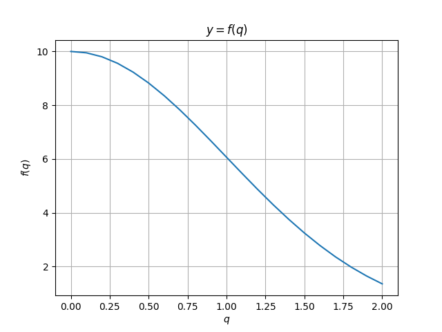
Consider the model of behavior on the market of two competing firms producing similar goods in volumes x and y, enjoying unlimited demand [1]. We construct the following two functions for price and cost.
')
Listing of graphing functions of price and costs
# -*- coding: utf8 -*- import numpy as np import matplotlib.pyplot as plt a=10 def f(q): return a*np.e**(-0.5*q**2) def h(q): # return np.sqrt(q) plt.figure() q= np.arange(0, 2.01, 0.1)# plt.title(r'$y=f(q)$') # TeX plt.ylabel(r'$f(q)$') # y TeX plt.xlabel(r'$q$') # x TeX plt.grid(True) # plt.plot(q,f(q)) # plt.figure() plt.title(r'$y=h(q)$') # TeX plt.ylabel(r'$h(q)$') # y TeX plt.xlabel(r'$q$') # x TeX plt.grid(True) # plt.plot(q,h(q)) # plt.show() # Graph of price versus volume of goods sold
Graph of the dependence of costs on the volume of goods sold
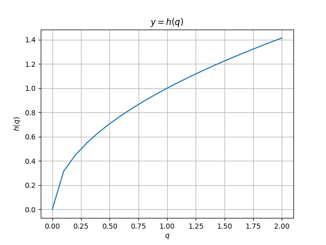
The price of the proposed product is characterized by a decreasing function f (q) of the volume of goods sold q = x + y. Costs production costs are the same for both firms and represent an increasing function h1 (x) = h2 (x) = h (x) .
Behavioral characteristics of two competing firms in the market
In the above conditions, the profit of each company is determined by the following functions:
L1 (x, y) = x * f (x + y) -h (x) L2 (x, y) = y * f (x + y) -h (y)
Consider the various behaviors of competitors in terms of game theory.
A. Let there be a zero-sum game with the first player's win:
L1 (x, y) = x * f (x + y) -h (x)
The goal of the second player is to minimize the profits of the first company for its ruin, i.e. need to find:
maxmin L (x, y) = maxmin x * f (x + y) -h (x)
xyxy
Let us reduce the game to the matrix, presenting the strategies of both players in a discrete form: xi = i * x1, yj = j * h2, i, j = 0 ... N. Its solution is given in the following listing:
Program Listing - Behavior Strategy A
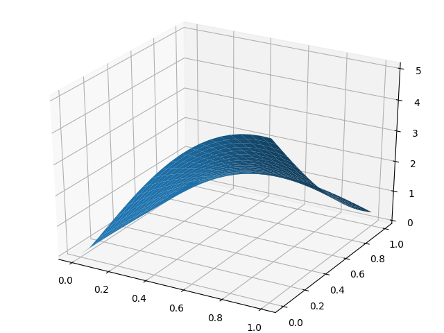
# -*- coding: utf8 -*- import pylab from mpl_toolkits.mplot3d import Axes3D import numpy as np xmax=1;ymax=1;N=20; h1=xmax/N;h2=ymax/N# def L1(x,y):# return 10*x*np.e**(-0.5*(x+y)**2)-np.sqrt(x) def L2(x,y):# return 10*y*np.e**(-0.5*(x+y)**2)-np.sqrt(y) def fi(a,b):# for w in range(0,len(a)+1): if a[w]==b: return w L= np.zeros([N+1,N+1])# for i in range(0,N+1): for j in range(0,N+1): L[i,j]=L1(i*h1,j*h2) A=[];e=[] rows, cols = L.shape for i in range(rows): e=[] for j in range(cols): e.append(L[i,j]) A.append(min(e)) a=max(A);ia=fi(A,a);xa=ia*h1# B=[];e=[] rows, cols = L.shape for j in range(cols): e=[] for i in range(rows): e.append(L[i,j]) B.append(max(e)) b=min(B);ib=fi(B,b);yb=ib*h2# p1=round(L1(xa,yb),3) print(" -"+str(p1)) p2=round(L2(xa,yb),3) print(" -"+str(p2)) def makeData_L1 ():# - z, - x,y x=[h1*i for i in np.arange(0,N+1)] y=[h2*i for i in np.arange(0,N+1)] x,y= np.meshgrid(x, y) z=[] for i in range(0,N+1): z.append(L1(x[i],y[i])) return x, y, z fig = pylab.figure() axes = Axes3D(fig) x, y, z = makeData_L1() axes.plot_surface(x, y, z) def makeData_L2 ():# - z - x,y x=[h1*i for i in np.arange(0,N+1)] y=[h2*i for i in np.arange(0,N+1)] x,y= np.meshgrid(x, y) z=[] for i in range(0,N+1): z.append(L2(x[i],y[i])) return x, y, z fig = pylab.figure() axes = Axes3D(fig) x, y, z = makeData_L2() axes.plot_surface(x, y, z) pylab.show() The results of the program:
Profit of the first company -0.916
The profit of the second company -2.247
Surface profit - z, purchase volumes - x, y for the first company
Surface profit - z, purchase volumes - x, y for the second company
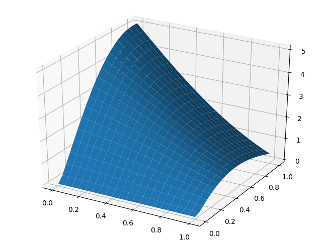
In accordance with this decision, the second player must maintain maximum sales in order to reduce prices and minimize the profits of the first player. The first player finds the optimal production volume under these conditions, however, he receives less profit than the second player.
B. If the first player is not satisfied with this situation, he can also set himself the goal of ruining the second player. If they change places, then due to the symmetry of the functions, the optimal strategy of the first player becomes optimal for the second player, and vice versa. If everyone wants to destroy a competitor, he must maximize the release of their goods.
Program Listing - Behavior Strategy B
# -*- coding: utf8 -*- import pylab import numpy as np xmax=1;ymax=1;N=20; h1=xmax/N;h2=ymax/N def L1(x,y): return 10*x*np.e**(-0.5*(x+y)**2)-np.sqrt(x) print(" -"+str(round(L1(xmax,ymax),3))) The result of the program
Profit of everyone with strategy B -0.353
With strategy B, each of the market participants will receive a profit of L1 = 0.353 , which is less for each player than in case A.
C. If competitors can agree on a market division, then they can achieve the most profitable result for each of them with a profit of 2,236 units, as shown in the following Python listing.
Program Listing - Behavior Strategy C
# -*- coding: utf8 -*- import matplotlib.pyplot as plt import numpy as np xmax=1;ymax=1;N=20; h1=xmax/N;h2=ymax/N def L1(x,y): return 10*x*np.e**(-0.5*(x+y)**2)-np.sqrt(x) z=[L1(i*h1,i*h1)for i in np.arange(0,N+1)] x=[h1*i for i in np.arange(0,N+1)] xopt=x[z.index(max(z))] print(" -"+str(xopt)) print(" -"+str(round(max(z),3))) plt.title(' ') plt.grid(True) plt.plot(x,z) plt.show() The result of the program:
The volume of goods of each company at which -0.45 is reached
The profit of each company -2.331

Conclusion
In a strategic game, the operating side counts on the most unfavorable case for itself, which comes down to calculating the operations of minimax and maximin. The implementation of this approach in Python expands the possibilities of creating game problems related to the optimization of economic systems.
Thank you all for your attention!
Links
1. Optimization of economic systems. mathcad examples and algorithms.
Source: https://habr.com/ru/post/335972/
All Articles