Description of sorting algorithms and comparison of their performance
Introduction
Many articles have already been written on this topic. However, I have not yet seen the article, which compares all the basic sorting on a large number of tests of different types and sizes. In addition, the implementation and description of the test suite are far from being everywhere. This leads to the fact that there may be doubts about the correctness of the study. However, the goal of my work is not only to determine which sorts work the fastest (in general, this is already known). First of all, I was interested in exploring algorithms, optimizing them so that they work as quickly as possible. Working on this, I managed to come up with an effective formula for sorting Shell.
In many ways, the article is devoted to how to write all the algorithms and test them. If we talk about programming itself, sometimes unexpected difficulties may arise (largely due to the C ++ optimizer). However, it is equally difficult to decide which tests exactly and in what quantities should be done. Codes of all algorithms that are laid out in this article, written by me. Run results are available on all tests. The only thing I can’t show is the tests themselves, since they weigh almost 140 GB. At the slightest suspicion, I checked both the code corresponding to the test and the test itself. I hope you enjoy the article.
Description of the main sorts and their implementation
I will try to briefly and clearly describe the sorting and specify the asymptotics, although the latter is not very important in the framework of this article (it is interesting to know the real time of work). I will not write anything about memory consumption in the future, I will only note that sortings that use complicated data structures (such as tree sorting) usually consume it in large quantities, and other sortings in the worst case only create an auxiliary array. There is also the concept of stability (sustainability) sorting. This means that the relative order of elements does not change when they are equal. This is also unimportant within the framework of this article (after all, you can simply attach an index to an element), but it will be useful in one place.
Bubble sort
We will go through the array from left to right. If the current item is greater than the next one, swap them. Do this until the array is sorted. Note that after the first iteration, the largest element will be at the end of the array, in the right place. After two iterations, the two largest elements will stand in the right place, and so on. Obviously, no more than after n iterations the array will be sorted. Thus, the asymptotics in the worst and average case is O (n 2 ), at best O (n).
')
Implementation:
void bubblesort(int* l, int* r) { int sz = r - l; if (sz <= 1) return; bool b = true; while (b) { b = false; for (int* i = l; i + 1 < r; i++) { if (*i > *(i + 1)) { swap(*i, *(i + 1)); b = true; } } r--; } } Shaker sort / Shaker sort
(also known as mixing and cocktail sorting). Note that bubble sorting works slowly on tests, in which small elements stand at the end (they are also called “turtles”). Such an element at each step of the algorithm will move only one position to the left. Therefore, we will go not only from left to right, but also from right to left. We will support two pointers begin and end, denoting which segment of the array has not yet been sorted. At the next iteration, when reaching end, subtract a unit from it and move from right to left, similarly, when you reach begin, add one and move from left to right. The asymptotics of the algorithm is the same as that of bubble sorting, but the real time is better.
Implementation:
void shakersort(int* l, int* r) { int sz = r - l; if (sz <= 1) return; bool b = true; int* beg = l - 1; int* end = r - 1; while (b) { b = false; beg++; for (int* i = beg; i < end; i++) { if (*i > *(i + 1)) { swap(*i, *(i + 1)); b = true; } } if (!b) break; end--; for (int* i = end; i > beg; i--) { if (*i < *(i - 1)) { swap(*i, *(i - 1)); b = true; } } } } Comb sort
Another modification of the sorting bubble. In order to get rid of "turtles", we will rearrange the elements that are at a distance. We fix it and we will go from left to right, comparing the elements standing at this distance, rearranging them, if necessary. Obviously, this will allow "turtles" to quickly get to the beginning of the array. It is optimal to initially take the distance equal to the length of the array, and then divide it by some coefficient equal to about 1.247. When the distance is equal to one, the bubble is sorted. At best, the asymptotics is O (nlogn), at worst, O (n 2 ). What is the average asymptotics for me is not very clear;
Implementation:
void combsort(int* l, int* r) { int sz = r - l; if (sz <= 1) return; double k = 1.2473309; int step = sz - 1; while (step > 1) { for (int* i = l; i + step < r; i++) { if (*i > *(i + step)) swap(*i, *(i + step)); } step /= k; } bool b = true; while (b) { b = false; for (int* i = l; i + 1 < r; i++) { if (*i > *(i + 1)) { swap(*i, *(i + 1)); b = true; } } } } You can also read about these sortings (bubble, shaker and comb) here .
Sort Inserts / Insertion sort
Let's create an array in which after the completion of the algorithm will be the answer. Let us alternately insert elements from the source array so that the elements in the response array are always sorted. The average and worst case asymptotics is O (n 2 ); at best, O (n). It is more convenient to implement the algorithm in a different way (creating a new array and actually inserting something into it is relatively difficult): we simply make sure that some prefix of the original array is sorted, instead of inserting, we will change the current element with the previous one while they are in the wrong order.
Implementation:
void insertionsort(int* l, int* r) { for (int *i = l + 1; i < r; i++) { int* j = i; while (j > l && *(j - 1) > *j) { swap(*(j - 1), *j); j--; } } } Shellsort
Use the same idea as sorting with a comb, and apply to sorting inserts. Fix some distance. Then the elements of the array will be divided into classes — elements fall into one class, the distance between which is a multiple of the fixed distance. Sort by insertion sorting each class. Unlike the sorting comb, the optimal set of distances is unknown. There are quite a few sequences with different ratings. Shell sequence - the first element is equal to the length of the array, each following one half the previous one. In the worst case, the asymptotics is O (n 2 ). Hibbard sequence - 2 n - 1, asymptotics in the worst case - O (n 1,5 ), Sedgwik sequence (the formula is nontrivial, you can see it by the link below) - O (n 4/3 ), Pratt (all products of powers of two and triples) - O (nlog 2 n). I note that all these sequences need to be calculated only to the size of the array and run from the larger one to the smaller one (otherwise, it will just be sorting by inserts). I also conducted additional research and tested different sequences of the form s i = a * s i - 1 + k * s i - 1 (partly this was inspired by the empirical Tsiura sequence - one of the best distance sequences for a small number of elements). The best were sequences with coefficients a = 3, k = 1/3; a = 4, k = 1/4 and a = 4, k = -1/5.
Some useful links:
Sorting Shell in Russian Wikipedia
Sort Shell in English Wikipedia
Article on Habré
Implementations:
void shellsort(int* l, int* r) { int sz = r - l; int step = sz / 2; while (step >= 1) { for (int *i = l + step; i < r; i++) { int *j = i; int *diff = j - step; while (diff >= l && *diff > *j) { swap(*diff, *j); j = diff; diff = j - step; } } step /= 2; } } void shellsorthib(int* l, int* r) { int sz = r - l; if (sz <= 1) return; int step = 1; while (step < sz) step <<= 1; step >>= 1; step--; while (step >= 1) { for (int *i = l + step; i < r; i++) { int *j = i; int *diff = j - step; while (diff >= l && *diff > *j) { swap(*diff, *j); j = diff; diff = j - step; } } step /= 2; } } int steps[100]; void shellsortsedgwick(int* l, int* r) { int sz = r - l; steps[0] = 1; int q = 1; while (steps[q - 1] * 3 < sz) { if (q % 2 == 0) steps[q] = 9 * (1 << q) - 9 * (1 << (q / 2)) + 1; else steps[q] = 8 * (1 << q) - 6 * (1 << ((q + 1) / 2)) + 1; q++; } q--; for (; q >= 0; q--) { int step = steps[q]; for (int *i = l + step; i < r; i++) { int *j = i; int *diff = j - step; while (diff >= l && *diff > *j) { swap(*diff, *j); j = diff; diff = j - step; } } } } void shellsortpratt(int* l, int* r) { int sz = r - l; steps[0] = 1; int cur = 1, q = 1; for (int i = 1; i < sz; i++) { int cur = 1 << i; if (cur > sz / 2) break; for (int j = 1; j < sz; j++) { cur *= 3; if (cur > sz / 2) break; steps[q++] = cur; } } insertionsort(steps, steps + q); q--; for (; q >= 0; q--) { int step = steps[q]; for (int *i = l + step; i < r; i++) { int *j = i; int *diff = j - step; while (diff >= l && *diff > *j) { swap(*diff, *j); j = diff; diff = j - step; } } } } void myshell1(int* l, int* r) { int sz = r - l, q = 1; steps[0] = 1; while (steps[q - 1] < sz) { int s = steps[q - 1]; steps[q++] = s * 4 + s / 4; } q--; for (; q >= 0; q--) { int step = steps[q]; for (int *i = l + step; i < r; i++) { int *j = i; int *diff = j - step; while (diff >= l && *diff > *j) { swap(*diff, *j); j = diff; diff = j - step; } } } } void myshell2(int* l, int* r) { int sz = r - l, q = 1; steps[0] = 1; while (steps[q - 1] < sz) { int s = steps[q - 1]; steps[q++] = s * 3 + s / 3; } q--; for (; q >= 0; q--) { int step = steps[q]; for (int *i = l + step; i < r; i++) { int *j = i; int *diff = j - step; while (diff >= l && *diff > *j) { swap(*diff, *j); j = diff; diff = j - step; } } } } void myshell3(int* l, int* r) { int sz = r - l, q = 1; steps[0] = 1; while (steps[q - 1] < sz) { int s = steps[q - 1]; steps[q++] = s * 4 - s / 5; } q--; for (; q >= 0; q--) { int step = steps[q]; for (int *i = l + step; i < r; i++) { int *j = i; int *diff = j - step; while (diff >= l && *diff > *j) { swap(*diff, *j); j = diff; diff = j - step; } } } } Sort tree / tree sort
We will insert elements into the binary search tree. After all the elements are inserted, it is enough to go around the tree to the depth and get a sorted array. If you use a balanced tree, such as red-black, the asymptotics will be equal to O (nlogn) in the worst, average and best. In the implementation used multiset container.
Here you can read about search trees:
Wikipedia
Article on Habré
And another article on Habré
Implementation:
void treesort(int* l, int* r) { multiset<int> m; for (int *i = l; i < r; i++) m.insert(*i); for (int q : m) *l = q, l++; } Gnome sort / Gnome sort
The algorithm is similar to sorting by inserts. We support the pointer to the current element, if it is greater than the previous one or it is the first one - move the pointer to the position to the right, otherwise we change the current and previous elements in places and move to the left.
Implementation:
void gnomesort(int* l, int* r) { int *i = l; while (i < r) { if (i == l || *(i - 1) <= *i) i++; else swap(*(i - 1), *i), i--; } } Sort selection / sort selection
At the next iteration, we will find the minimum in the array after the current element and change it with it if necessary. Thus, after the i-th iteration, the first i elements will stand in their places. Asymptotics: O (n 2 ) at best, average and worst. It should be noted that this sorting can be implemented in two ways - keeping the minimum and its index, or simply rearranging the current item with the item in question if they are in the wrong order. The first method was a little faster, so it is implemented.
Implementation:
void selectionsort(int* l, int* r) { for (int *i = l; i < r; i++) { int minz = *i, *ind = i; for (int *j = i + 1; j < r; j++) { if (*j < minz) minz = *j, ind = j; } swap(*i, *ind); } } Pyramid Sorting / Heapsort
Development of the idea of sorting choice We use the heap data structure (or “pyramid”, whence the name of the algorithm). It allows you to get at least O (1), adding elements and extracting at least O (logn). Thus, the asymptotic behavior of O (nlogn) is worst, average, and best. I implemented the heap myself, although in C ++ there is a container priority_queue, since this container is rather slow.
You can read about a bunch here:
Wikipedia
Article on Habré
Implementation:
template <class T> class heap { public: int size() { return n; } int top() { return h[0]; } bool empty() { return n == 0; } void push(T a) { h.push_back(a); SiftUp(n); n++; } void pop() { n--; swap(h[n], h[0]); h.pop_back(); SiftDown(0); } void clear() { h.clear(); n = 0; } T operator [] (int a) { return h[a]; } private: vector<T> h; int n = 0; void SiftUp(int a) { while (a) { int p = (a - 1) / 2; if (h[p] > h[a]) swap(h[p], h[a]); else break; a--; a /= 2; } } void SiftDown(int a) { while (2 * a + 1 < n) { int l = 2 * a + 1, r = 2 * a + 2; if (r == n) { if (h[l] < h[a]) swap(h[l], h[a]); break; } else if (h[l] <= h[r]) { if (h[l] < h[a]) { swap(h[l], h[a]); a = l; } else break; } else if (h[r] < h[a]) { swap(h[r], h[a]); a = r; } else break; } } }; void heapsort(int* l, int* r) { heap<int> h; for (int *i = l; i < r; i++) h.push(*i); for (int *i = l; i < r; i++) { *i = h.top(); h.pop(); } } Quick Sort / Quicksort
Choose some support element. After that, we will throw all the elements, the smaller ones, to the left, and the large ones - to the right. Recursively call from each of the parts. As a result, we obtain a sorted array, since each element of the smaller reference one was before each larger reference one. Asymptotics: O (nlogn) in the middle and best case, O (n 2 ). The worst estimate is achieved if the support element is unsuccessful. My implementation of this algorithm is completely standard, we go simultaneously to the left and to the right, we find a pair of elements such that the left element is larger than the reference element and the right element is smaller, and we swap them. In addition to pure quick sorting, the sorting was used in comparison, passing with a small number of elements on sorting by inserts. The constant is selected by testing, and the sorting by inserts is the best sorting suitable for this task (although it is not worth it to think that it is the fastest of quadratic ones).
Implementation:
void quicksort(int* l, int* r) { if (r - l <= 1) return; int z = *(l + (r - l) / 2); int* ll = l, *rr = r - 1; while (ll <= rr) { while (*ll < z) ll++; while (*rr > z) rr--; if (ll <= rr) { swap(*ll, *rr); ll++; rr--; } } if (l < rr) quicksort(l, rr + 1); if (ll < r) quicksort(ll, r); } void quickinssort(int* l, int* r) { if (r - l <= 32) { insertionsort(l, r); return; } int z = *(l + (r - l) / 2); int* ll = l, *rr = r - 1; while (ll <= rr) { while (*ll < z) ll++; while (*rr > z) rr--; if (ll <= rr) { swap(*ll, *rr); ll++; rr--; } } if (l < rr) quickinssort(l, rr + 1); if (ll < r) quickinssort(ll, r); } Merge sort / Merge sort
Sorting based on the divide-and-conquer paradigm. We divide the array in half, recursively sort the parts, and then execute the merge procedure: we support two pointers, one to the current element of the first part, the second to the current element of the second part. From these two elements, select the minimum, insert into the response and shift the pointer corresponding to the minimum. The merge works beyond O (n), the levels of all logn, so the asymptotics is O (nlogn). Effectively create a temporary array in advance and pass it as a function argument. This sorting is recursive, as well as quick, and therefore it is possible to switch to quadratic with a small number of elements.
Implementation:
void merge(int* l, int* m, int* r, int* temp) { int *cl = l, *cr = m, cur = 0; while (cl < m && cr < r) { if (*cl < *cr) temp[cur++] = *cl, cl++; else temp[cur++] = *cr, cr++; } while (cl < m) temp[cur++] = *cl, cl++; while (cr < r) temp[cur++] = *cr, cr++; cur = 0; for (int* i = l; i < r; i++) *i = temp[cur++]; } void _mergesort(int* l, int* r, int* temp) { if (r - l <= 1) return; int *m = l + (r - l) / 2; _mergesort(l, m, temp); _mergesort(m, r, temp); merge(l, m, r, temp); } void mergesort(int* l, int* r) { int* temp = new int[r - l]; _mergesort(l, r, temp); delete temp; } void _mergeinssort(int* l, int* r, int* temp) { if (r - l <= 32) { insertionsort(l, r); return; } int *m = l + (r - l) / 2; _mergeinssort(l, m, temp); _mergeinssort(m, r, temp); merge(l, m, r, temp); } void mergeinssort(int* l, int* r) { int* temp = new int[r - l]; _mergeinssort(l, r, temp); delete temp; } Sort by Counting / Counting sort
Create an array of size r - l, where l is the minimum and r is the maximum element of the array. After that, go through the array and count the number of occurrences of each element. Now you can go through the array of values and write out each number as many times as necessary. Asymptotics - O (n + r - l). You can modify this algorithm so that it becomes stable: to do this, we define the place where the next number should be (this is just the prefix sums in the array of values) and we will go through the source array from left to right, putting the element in the right place and increasing the position by 1. This the sorting was not tested, since most of the tests contained rather large numbers that did not allow to create an array of the required size. However, it nevertheless came in handy.
Block Sort / Bucket sort
(also known as basket and pocket sorting). Let l be the minimal and r the maximal element of the array. We divide the elements into blocks, in the first there will be elements from l to l + k, in the second - from l + k to l + 2k, etc., where k = (r - l) / number of blocks. In general, if the number of blocks is two, then this algorithm turns into a sort of quick sort. The asymptotics of this algorithm is unclear, the running time depends on the input data and the number of blocks. It is argued that on successful data, the operating time is linear. The implementation of this algorithm turned out to be one of the most difficult tasks. You can do it this way: just create new arrays, recursively sort and glue them. However, this approach is still rather slow and did not suit me. In an effective implementation, several ideas are used:
1) We will not create new arrays. To do this, we use the sorting counting technique - we calculate the number of elements in each block, the prefix sums and, thus, the position of each element in the array.
2) We will not run from empty blocks. Put the indices of non-empty blocks in a separate array and run only on them.
3) Check whether the array is sorted. This does not worsen the running time, since you still need to make a pass in order to find the minimum and maximum, however, it will allow the algorithm to speed up on partially sorted data, because the elements are inserted into new blocks in the same order as in the original array.
4) Since the algorithm turned out to be rather cumbersome, with a small number of elements it is extremely inefficient. To such an extent that the transition to sorting inserts speeds up the work by about 10 times.
It remains only to understand how many blocks you need to choose. On randomized tests, I managed to get the following grade: 1500 units for 10 7 elements and 3000 for 10 8 . It was not possible to pick up the formula - the work time deteriorated several times.
Implementation:
void _newbucketsort(int* l, int* r, int* temp) { if (r - l <= 64) { insertionsort(l, r); return; } int minz = *l, maxz = *l; bool is_sorted = true; for (int *i = l + 1; i < r; i++) { minz = min(minz, *i); maxz = max(maxz, *i); if (*i < *(i - 1)) is_sorted = false; } if (is_sorted) return; int diff = maxz - minz + 1; int numbuckets; if (r - l <= 1e7) numbuckets = 1500; else numbuckets = 3000; int range = (diff + numbuckets - 1) / numbuckets; int* cnt = new int[numbuckets + 1]; for (int i = 0; i <= numbuckets; i++) cnt[i] = 0; int cur = 0; for (int* i = l; i < r; i++) { temp[cur++] = *i; int ind = (*i - minz) / range; cnt[ind + 1]++; } int sz = 0; for (int i = 1; i <= numbuckets; i++) if (cnt[i]) sz++; int* run = new int[sz]; cur = 0; for (int i = 1; i <= numbuckets; i++) if (cnt[i]) run[cur++] = i - 1; for (int i = 1; i <= numbuckets; i++) cnt[i] += cnt[i - 1]; cur = 0; for (int *i = l; i < r; i++) { int ind = (temp[cur] - minz) / range; *(l + cnt[ind]) = temp[cur]; cur++; cnt[ind]++; } for (int i = 0; i < sz; i++) { int r = run[i]; if (r != 0) _newbucketsort(l + cnt[r - 1], l + cnt[r], temp); else _newbucketsort(l, l + cnt[r], temp); } delete run; delete cnt; } void newbucketsort(int* l, int* r) { int *temp = new int[r - l]; _newbucketsort(l, r, temp); delete temp; } Bitwise sort / Radix sort
(also known as digital sorting). There are two versions of this sorting, in which, in my opinion, there is little in common, apart from the idea of using the representation of a number in some number system (for example, binary).
LSD (least significant digit):
Imagine each number in binary form. At each step of the algorithm, we will sort the numbers so that they are sorted by the first k * i bits, where k is some constant. From this definition, it follows that at each step it is sufficient to stably sort the elements by the new k bits. Sorting by counting is ideal for this (2 k of memory and time are needed, which is a bit with a successful choice of a constant). Asymptotics: O (n), if we assume that the numbers are of a fixed size (and otherwise it would not be possible to assume that the comparison of two numbers is performed per unit time). The implementation is quite simple.
Implementation:
int digit(int n, int k, int N, int M) { return (n >> (N * k) & (M - 1)); } void _radixsort(int* l, int* r, int N) { int k = (32 + N - 1) / N; int M = 1 << N; int sz = r - l; int* b = new int[sz]; int* c = new int[M]; for (int i = 0; i < k; i++) { for (int j = 0; j < M; j++) c[j] = 0; for (int* j = l; j < r; j++) c[digit(*j, i, N, M)]++; for (int j = 1; j < M; j++) c[j] += c[j - 1]; for (int* j = r - 1; j >= l; j--) b[--c[digit(*j, i, N, M)]] = *j; int cur = 0; for (int* j = l; j < r; j++) *j = b[cur++]; } delete b; delete c; } void radixsort(int* l, int* r) { _radixsort(l, r, 8); } MSD (most significant digit):
In fact, some kind of block sorting. Numbers with equal k bits will fall into one block. Asymptotics is the same as for LSD version. The implementation is very similar to block sorting, but simpler. It uses the digit function defined in the LSD version implementation.
Implementation:
void _radixsortmsd(int* l, int* r, int N, int d, int* temp) { if (d == -1) return; if (r - l <= 32) { insertionsort(l, r); return; } int M = 1 << N; int* cnt = new int[M + 1]; for (int i = 0; i <= M; i++) cnt[i] = 0; int cur = 0; for (int* i = l; i < r; i++) { temp[cur++] = *i; cnt[digit(*i, d, N, M) + 1]++; } int sz = 0; for (int i = 1; i <= M; i++) if (cnt[i]) sz++; int* run = new int[sz]; cur = 0; for (int i = 1; i <= M; i++) if (cnt[i]) run[cur++] = i - 1; for (int i = 1; i <= M; i++) cnt[i] += cnt[i - 1]; cur = 0; for (int *i = l; i < r; i++) { int ind = digit(temp[cur], d, N, M); *(l + cnt[ind]) = temp[cur]; cur++; cnt[ind]++; } for (int i = 0; i < sz; i++) { int r = run[i]; if (r != 0) _radixsortmsd(l + cnt[r - 1], l + cnt[r], N, d - 1, temp); else _radixsortmsd(l, l + cnt[r], N, d - 1, temp); } delete run; delete cnt; } void radixsortmsd(int* l, int* r) { int* temp = new int[r - l]; _radixsortmsd(l, r, 8, 3, temp); delete temp; } Biton sort / Bitonic sort:
The idea of this algorithm is that the original array is converted into a biton sequence — a sequence that first grows and then decreases. It can be effectively sorted in the following way: we divide the array into two parts, create two arrays, add all elements equal to the minimum of the corresponding elements of each of the two parts to the first, and equal to the maximum in the second. It is argued that you get two bitonic sequences, each of which can be recursively sorted in the same way, after which you can glue two arrays (since any element of the first is less than or equal to any element of the second). In order to convert the original array into a biton sequence, we will do the following: if the array consists of two elements, you can simply complete, otherwise divide the array in half, recursively call the algorithm from the halves, then sort the first part in order, the second in reverse order and glue . Obviously, you get a biton sequence. Asymptotics: O (nlog 2 n), because when building the biton sequence we used the sorting working for O (nlogn), and logn was the whole level. Also note that the size of the array should be equal to the power of two, so you may have to supplement it with fictitious elements (which does not affect the asymptotics).
Implementation:
void bitseqsort(int* l, int* r, bool inv) { if (r - l <= 1) return; int *m = l + (r - l) / 2; for (int *i = l, *j = m; i < m && j < r; i++, j++) { if (inv ^ (*i > *j)) swap(*i, *j); } bitseqsort(l, m, inv); bitseqsort(m, r, inv); } void makebitonic(int* l, int* r) { if (r - l <= 1) return; int *m = l + (r - l) / 2; makebitonic(l, m); bitseqsort(l, m, 0); makebitonic(m, r); bitseqsort(m, r, 1); } void bitonicsort(int* l, int* r) { int n = 1; int inf = *max_element(l, r) + 1; while (n < r - l) n *= 2; int* a = new int[n]; int cur = 0; for (int *i = l; i < r; i++) a[cur++] = *i; while (cur < n) a[cur++] = inf; makebitonic(a, a + n); bitseqsort(a, a + n, 0); cur = 0; for (int *i = l; i < r; i++) *i = a[cur++]; delete a; } Timsort
Hybrid sorting, combining sorting inserts and merge sorting. We partition the array elements into several small subarrays, while expanding the subarray while the elements in it are sorted. We sort the subarrays by sorting by inserts, using the fact that it effectively works on sorted arrays. Next, we will merge the subarrays as in the merge sorting, taking them of approximately equal size (otherwise the work time will approach the quadratic one). For this, it is convenient to store subarrays in a stack, maintaining the invariant - the farther from the top, the larger the size, and merging the subarrays at the top only when the size of the third distant from the top of the subarray is greater than or equal to the sum of their sizes. Asymptotics: O (n) at best, and O (nlogn) at average and worst. The implementation is nontrivial,I have no firm confidence in it, however, she showed quite a good time and consistent with my ideas about how this sorting should work.
More timsort is described here:
Here
Here
Implementation:
void _timsort(int* l, int* r, int* temp) { int sz = r - l; if (sz <= 64) { insertionsort(l, r); return; } int minrun = sz, f = 0; while (minrun >= 64) { f |= minrun & 1; minrun >>= 1; } minrun += f; int* cur = l; stack<pair<int, int*>> s; while (cur < r) { int* c1 = cur; while (c1 < r - 1 && *c1 <= *(c1 + 1)) c1++; int* c2 = cur; while (c2 < r - 1 && *c2 >= *(c2 + 1)) c2++; if (c1 >= c2) { c1 = max(c1, cur + minrun - 1); c1 = min(c1, r - 1); insertionsort(cur, c1 + 1); s.push({ c1 - cur + 1, cur }); cur = c1 + 1; } else { c2 = max(c2, cur + minrun - 1); c2 = min(c2, r - 1); reverse(cur, c2 + 1); insertionsort(cur, c2 + 1); s.push({ c2 - cur + 1, cur }); cur = c2 + 1; } while (s.size() >= 3) { pair<int, int*> x = s.top(); s.pop(); pair<int, int*> y = s.top(); s.pop(); pair<int, int*> z = s.top(); s.pop(); if (z.first >= x.first + y.first && y.first >= x.first) { s.push(z); s.push(y); s.push(x); break; } else if (z.first >= x.first + y.first) { merge(y.second, x.second, x.second + x.first, temp); s.push(z); s.push({ x.first + y.first, y.second }); } else { merge(z.second, y.second, y.second + y.first, temp); s.push({ z.first + y.first, z.second }); s.push(x); } } } while (s.size() != 1) { pair<int, int*> x = s.top(); s.pop(); pair<int, int*> y = s.top(); s.pop(); if (x.second < y.second) swap(x, y); merge(y.second, x.second, x.second + x.first, temp); s.push({ y.first + x.first, y.second }); } } void timsort(int* l, int* r) { int* temp = new int[r - l]; _timsort(l, r, temp); delete temp; } Testing
Iron and system
Processor: Intel Core i7-3770 CPU 3.40 GHz
RAM: 8 GB
Testing was conducted on an almost pure Windows 10 x64 system installed a few days before launch. IDE used - Microsoft Visual Studio 2015.
Tests
All tests are divided into four groups. The first group is an array of random numbers in different modules (10, 1000, 10 5 , 10 7 and 10 9 ). The second group is an array broken into several sorted arrays. In fact, an array of random numbers was taken modulo 10 9, and then subarrays of size equal to the minimum of the length of the remaining suffix and a random number modulo some constant were sorted. The sequence of constants is 10, 100, 1000, etc. down to the size of the array. The third group is an initially sorted array of random numbers with a certain number of “swaps” - permutations of two random elements. The sequence of numbers of swaps is the same as in the previous group. Finally, the last group consists of several tests with a completely sorted array (in the direct and reverse order), several tests with an initial array of natural numbers from 1 to n, in which several numbers are replaced with a random one, and tests with a large number of repetitions of one element (10 %, 25%, 50%, 75% and 90%). Thus, tests allow you to seehow sorting works on random and partially sorted arrays, which looks the most significant. The fourth group is largely against linear-time sorts, which love random number sequences. At the end of the article there is a link to the file, which describes in detail all the tests.
It would be rather silly to compare, for example, sorting with linear time of work and quadratic, and run them on tests of the same size. Therefore, each of the groups of tests is divided into four groups, the size of 10 5 , 10 6 , 10 7 and 10 8 elements. The sortings were divided into three groups, in the first - quadratic (sorting by bubble, inserts, selection, shaker and gnomes), in the second - something between logarithmic time and square, (biton, several types of Shell sorting and sorting by tree), in the third all rest. Someone may be surprised that the tree sorting did not fall into the third group, although its asymptotics is O (nlogn), but, unfortunately, its constant is very large. Sorts of the first group were tested on tests with 105 elements, the second group - on tests with 10 6 and 10 7 , the third - on tests with 10 7 and 10 8 . It is these data sizes that allow you to somehow see an increase in the operating time, for smaller sizes the error is too large, for large ones the algorithm works too long (or lack of RAM). With the first group, I did not bother, so as not to disturb the tenfold increase (10 4 elements for quadratic sorts too little), after all, by themselves they are of little interest.
How was the testing done?
On each test, there were 20 launches, the total running time was an average of the resulting values. Almost all the results were obtained after one program launch, but due to several errors in the code and system glitches (testing lasted almost a week of pure time), some sortings and tests had to be retested afterwards.
Subtleties of implementation
It may be surprising to someone that I did not use function pointers in the implementation of the testing process itself, which would greatly reduce the code. It turned out that this significantly slows down the operation of the algorithm (approximately by 5-10%). Therefore, I used a separate call for each function (this, of course, would not affect the relative speed, but ... I still want to improve the absolute). For the same reason, vectors were replaced with regular arrays, patterns and comparators were not used. All this is more relevant for the industrial use of the algorithm, rather than testing it.
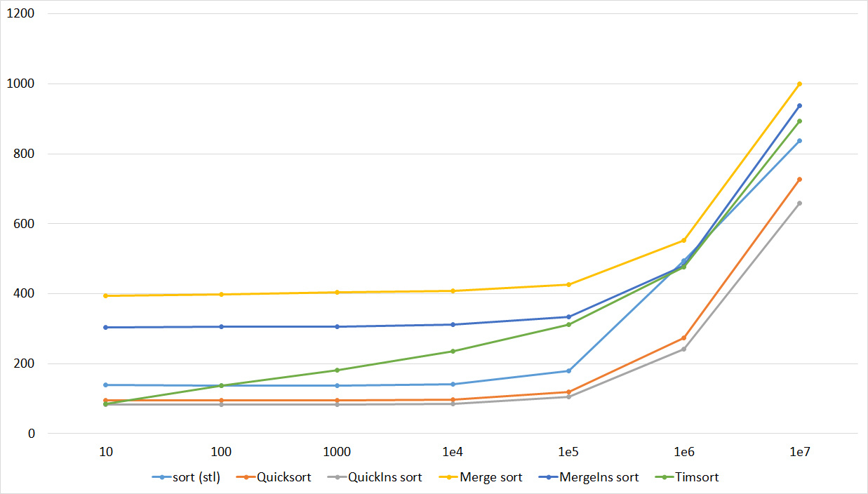
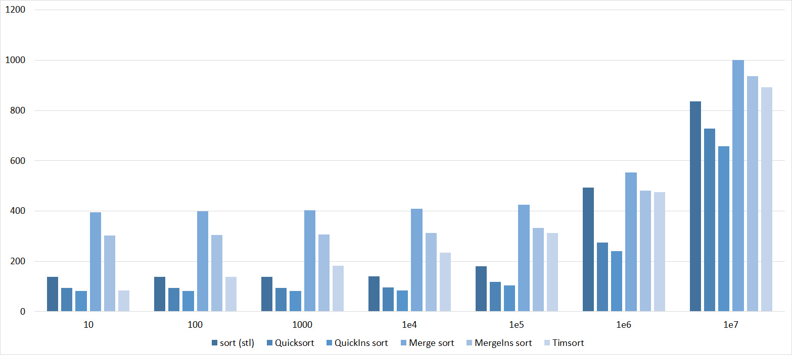
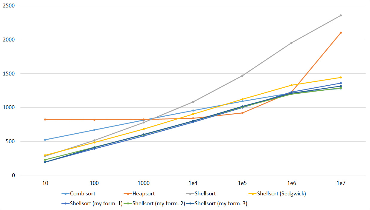
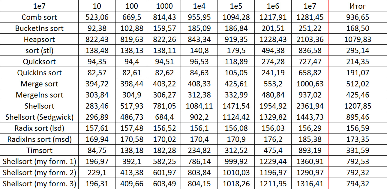
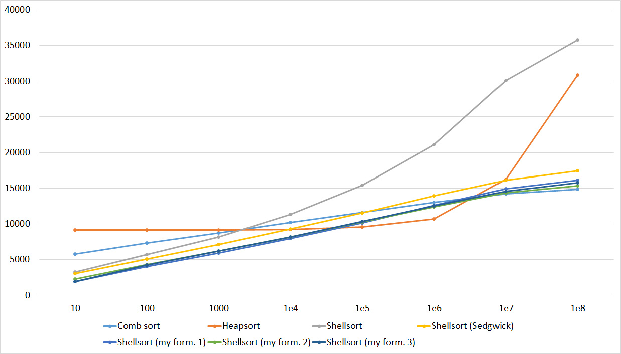
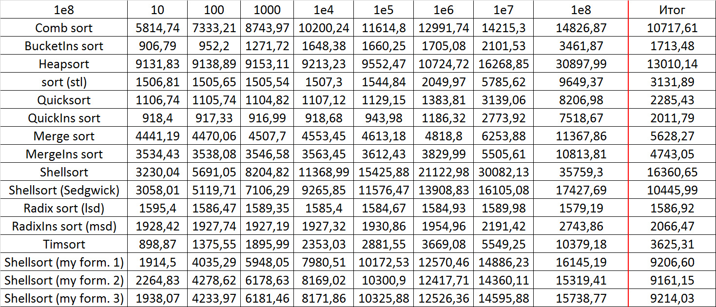
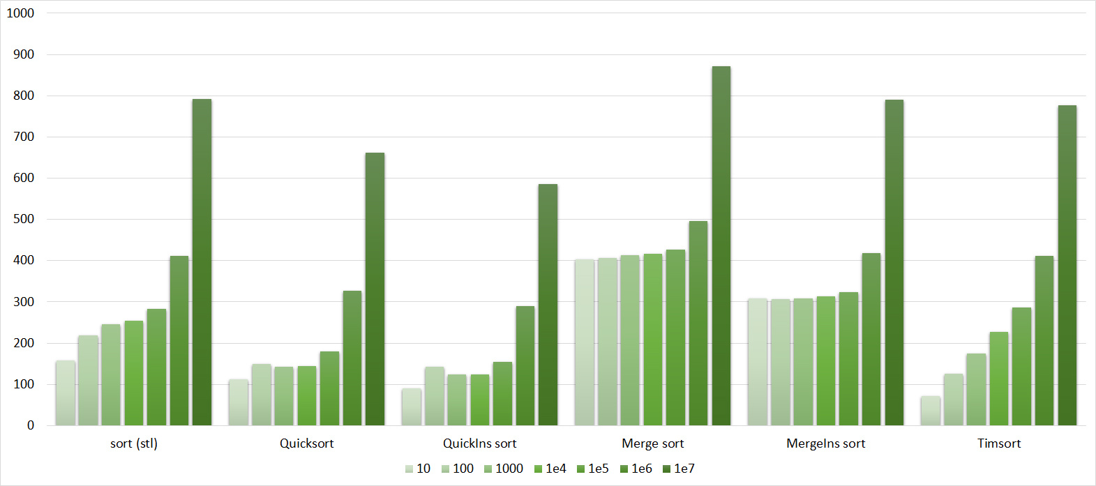
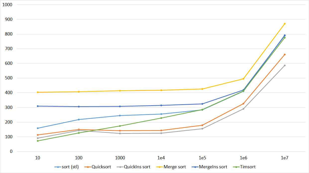
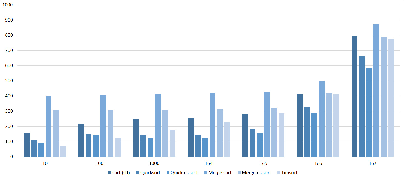
results
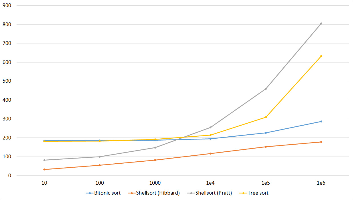
All results are available in several forms - three diagrams (a histogram showing the change in speed during the transition to the next constraint on one type of test, a graph depicting the same, but sometimes more clearly, and a histogram showing which sorting is best works on some type of test) and the table on which they are based. The third group was divided into three parts, but little would be clear. However, even so far not all diagrams are successful (in general, I strongly doubt the utility of the third type of diagrams), but I hope everyone can find the most suitable for understanding.
Since there are a lot of pictures, they are hidden by spoilers. Few comments about the notation. Sortings are named as above, if this is Shell sorting, then the author of the sequence is indicated in parentheses, Ins is assigned to the names of sortings that switch to sorting by inserts, (for compactness). In the diagrams for the second group of tests, the possible length of the sorted subarrays is indicated, for the third group - the number of swaps, for the fourth - the number of substitutions. The overall result was calculated as the average of four groups.
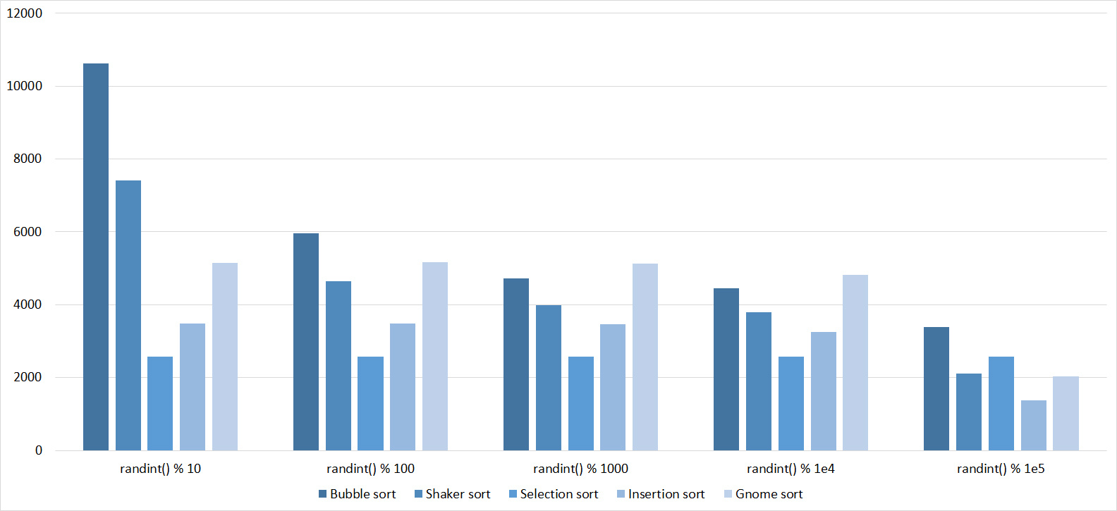
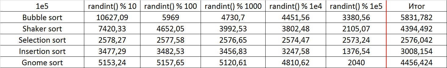
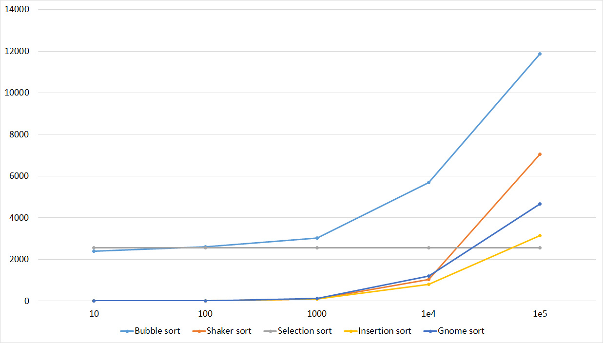
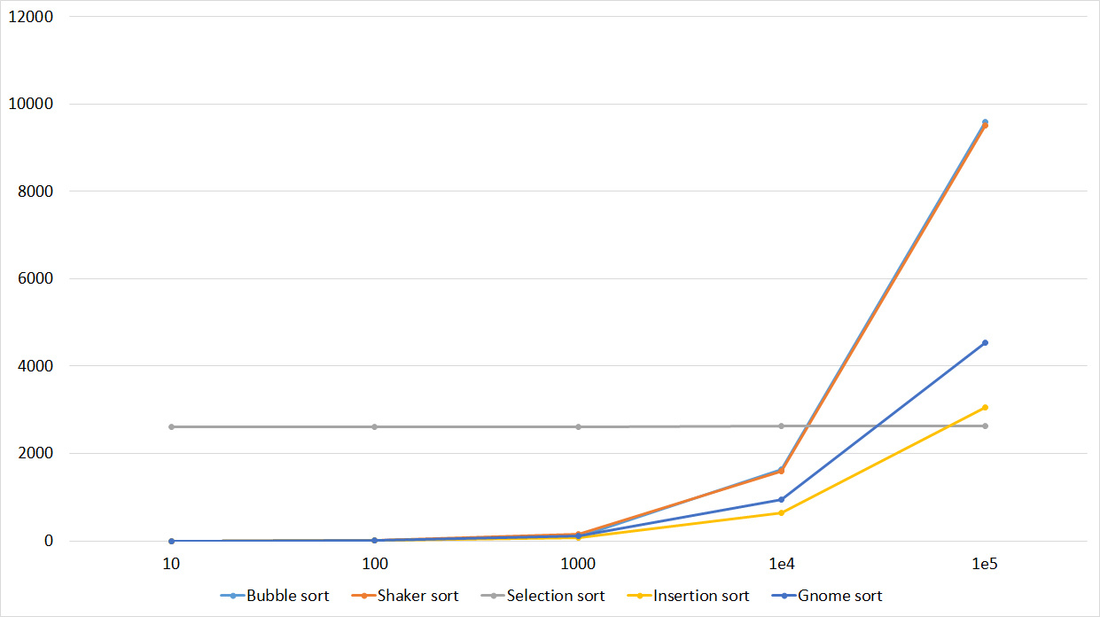
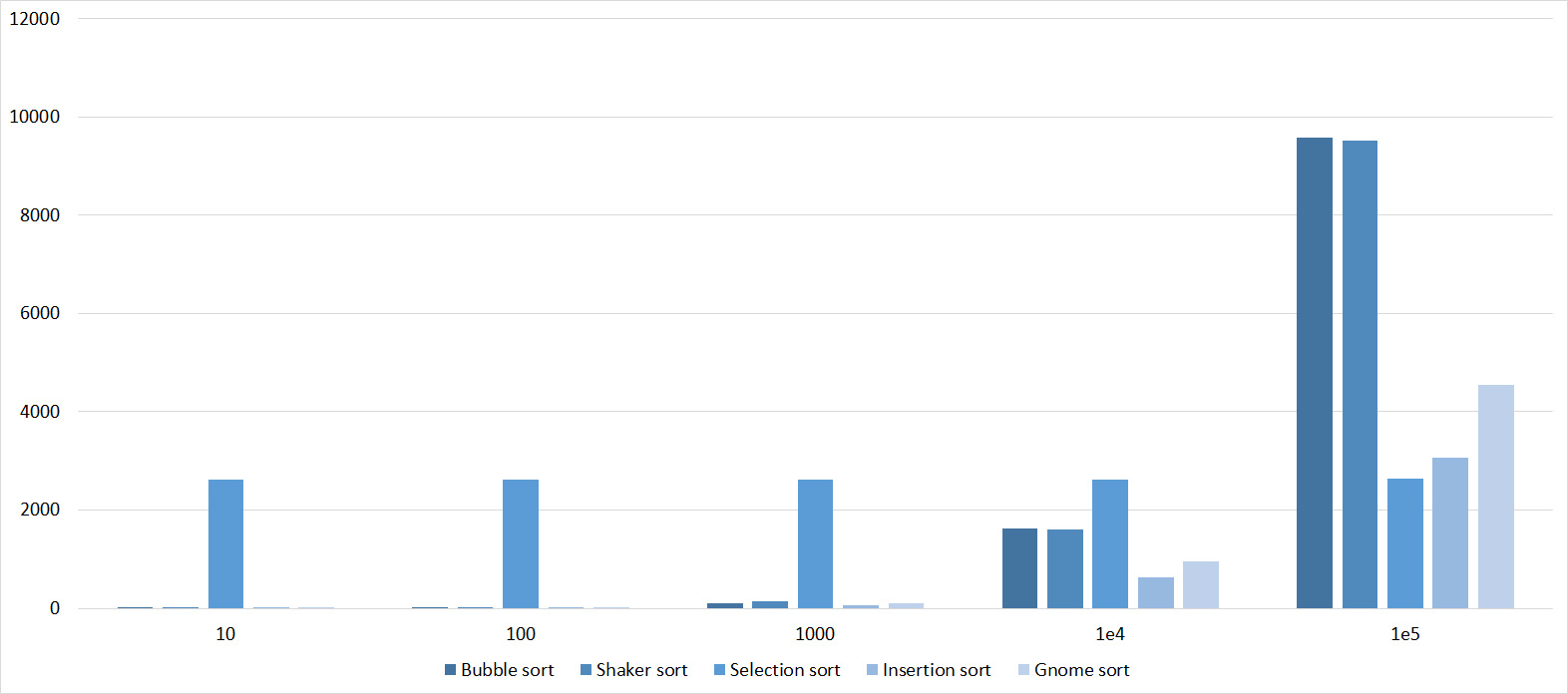
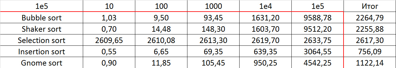
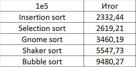
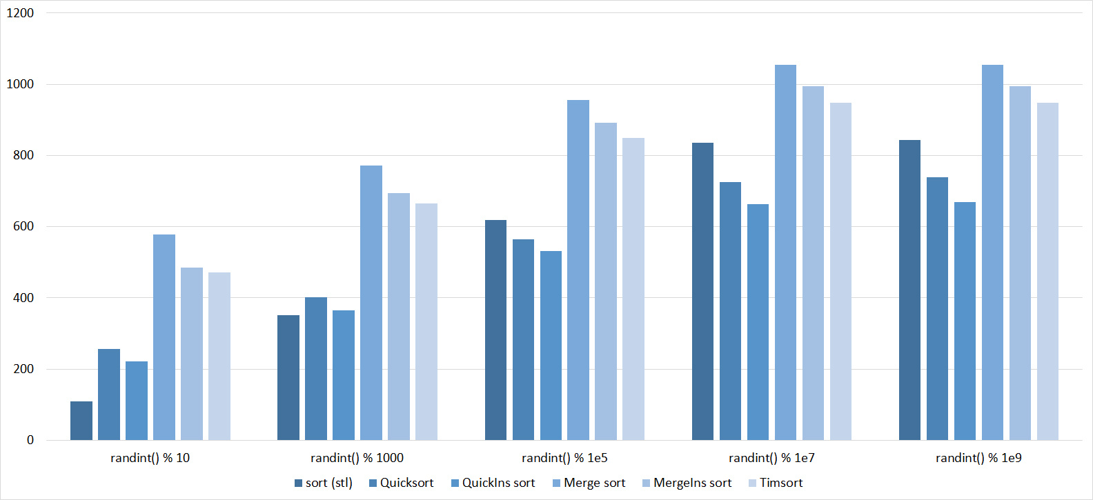
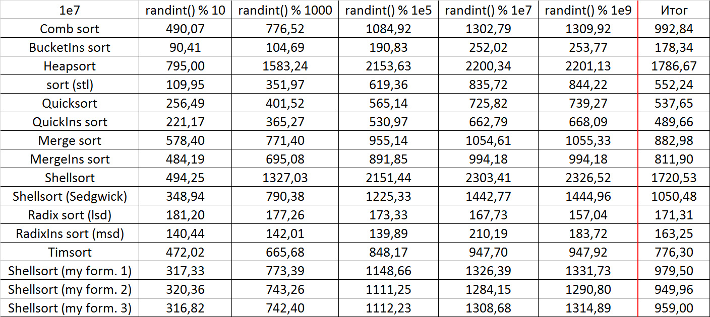
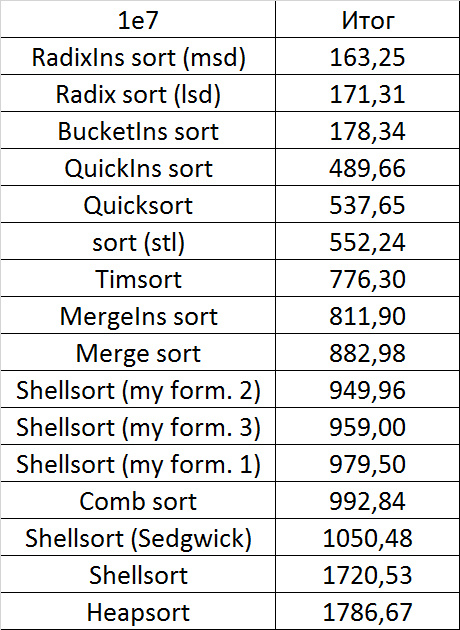
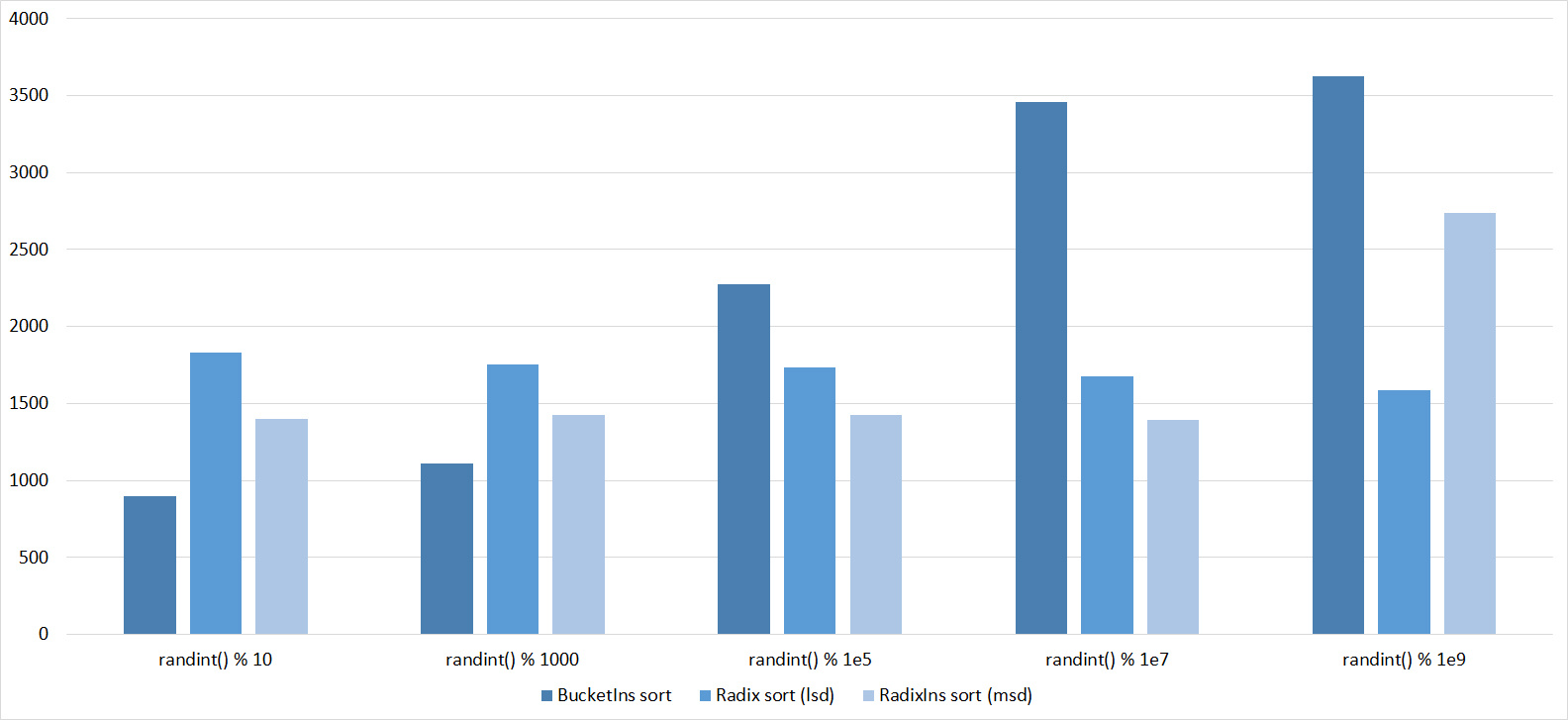
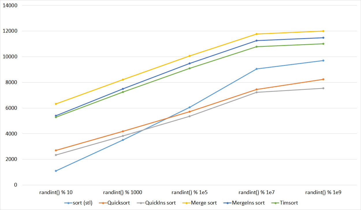
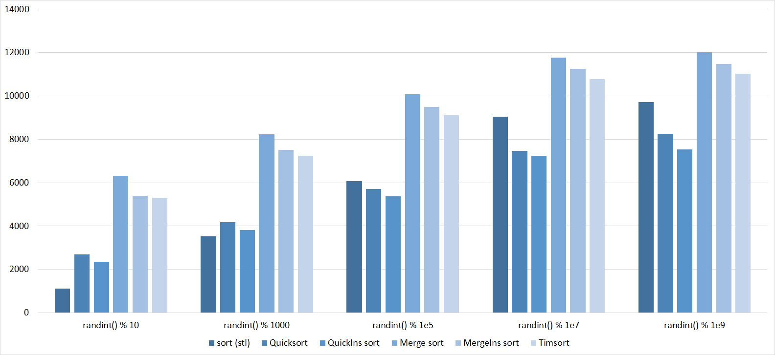
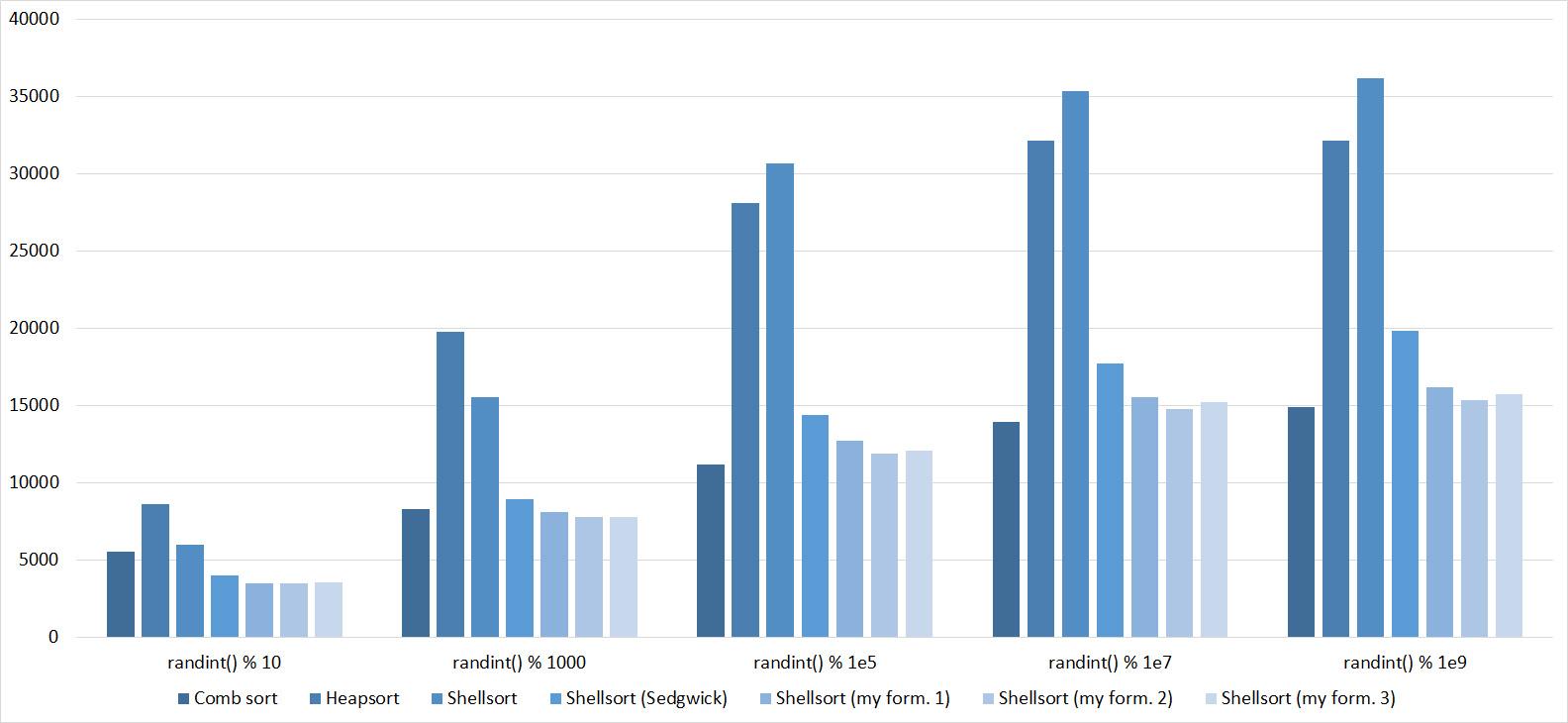
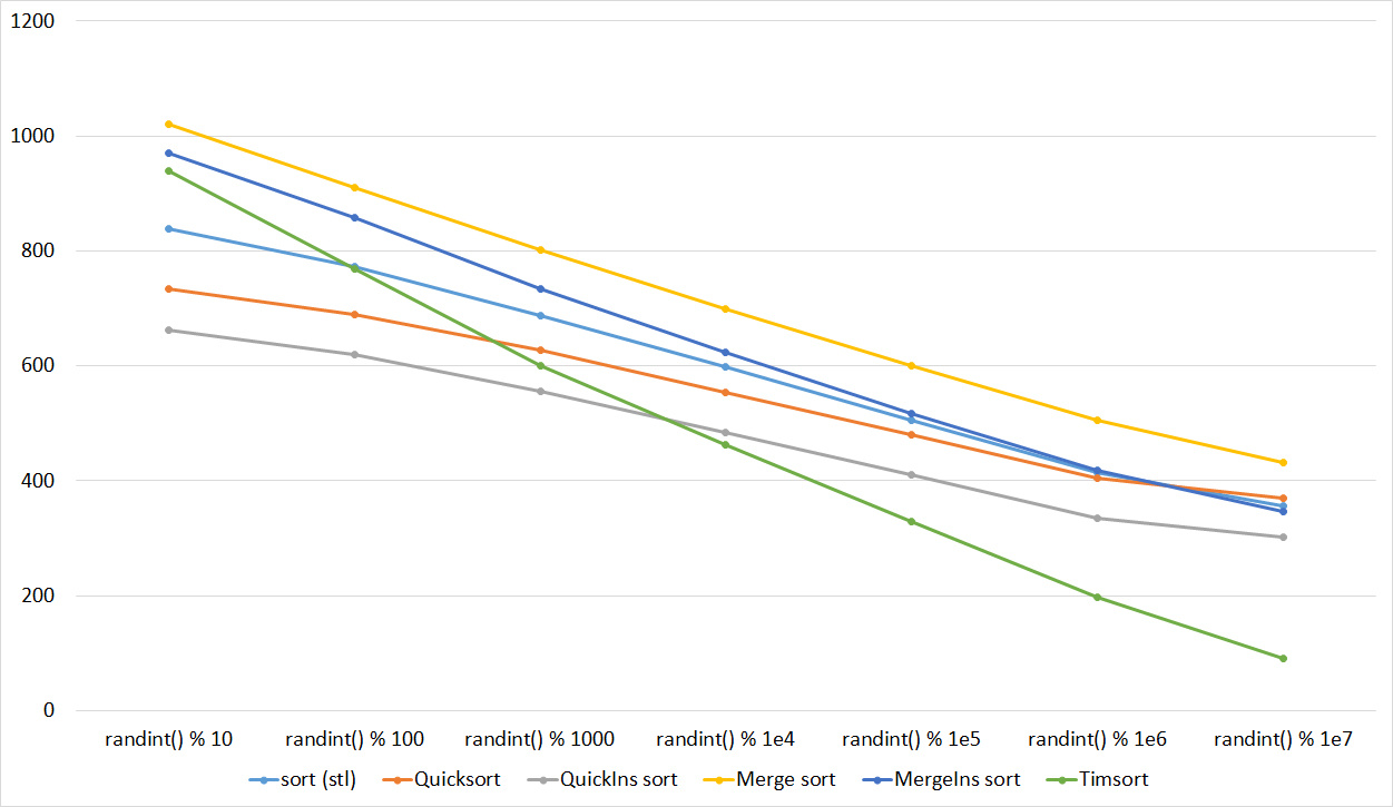
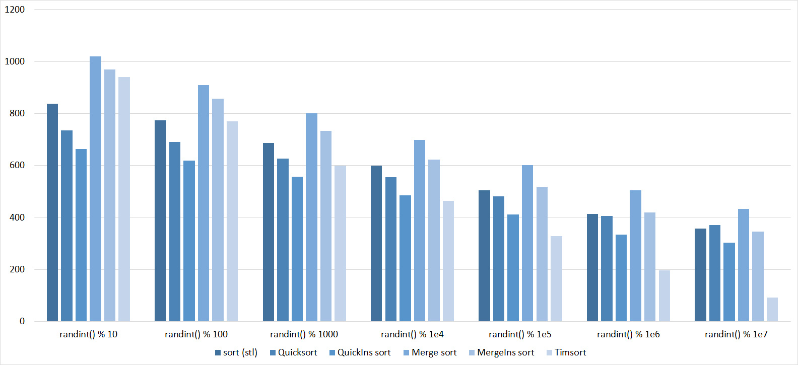
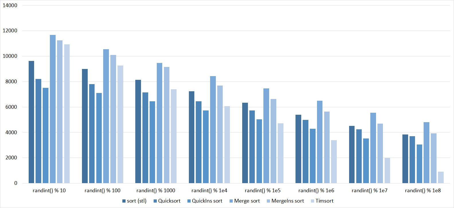
First Sort Group
Array of random numbers
Tables
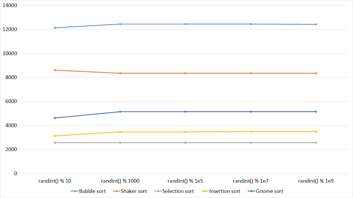


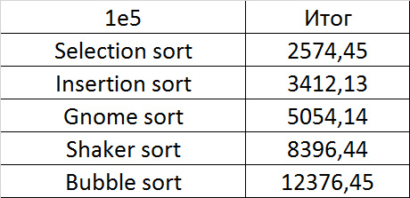
Very boring results, even partial sorting with a small module is almost imperceptible.
Partially sorted array
Tables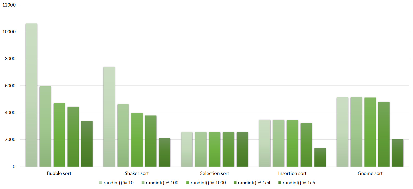
Already much more interesting. Exchange sorting the most rapidly responded, shaker even overtook Gnome. Sorting inserts sped up just at the very end. Sorting by choice, of course, works perfectly well.
Swaps
Tables


Here, sorting by inserts has finally manifested itself, although the increase in speed at the shaker is about the same. This showed a weak sorting bubble - one swap is enough, moving a small element to the end, and it is already running slowly. Sorting choice was almost at the end.
Permutation changes
Tables
The group is almost the same as the previous one, so the results are similar. However, the sorting of the bubble is pulled forward, since the random element inserted into the array will most likely be more than all the others, that is, in one iteration will move to the end. Sort by choice has become an outsider.
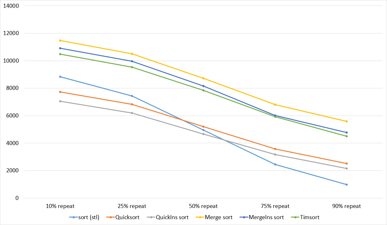
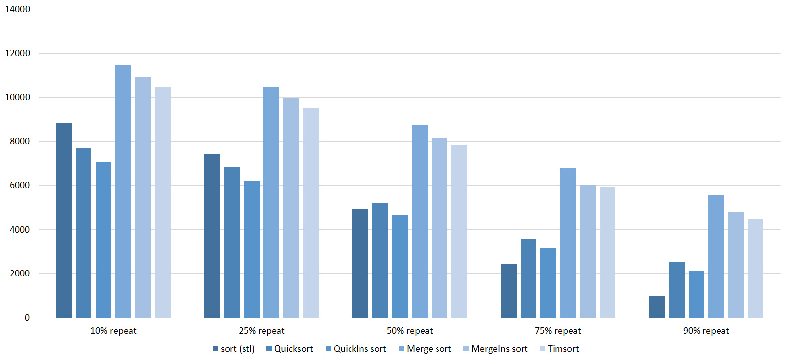
Replays
Tables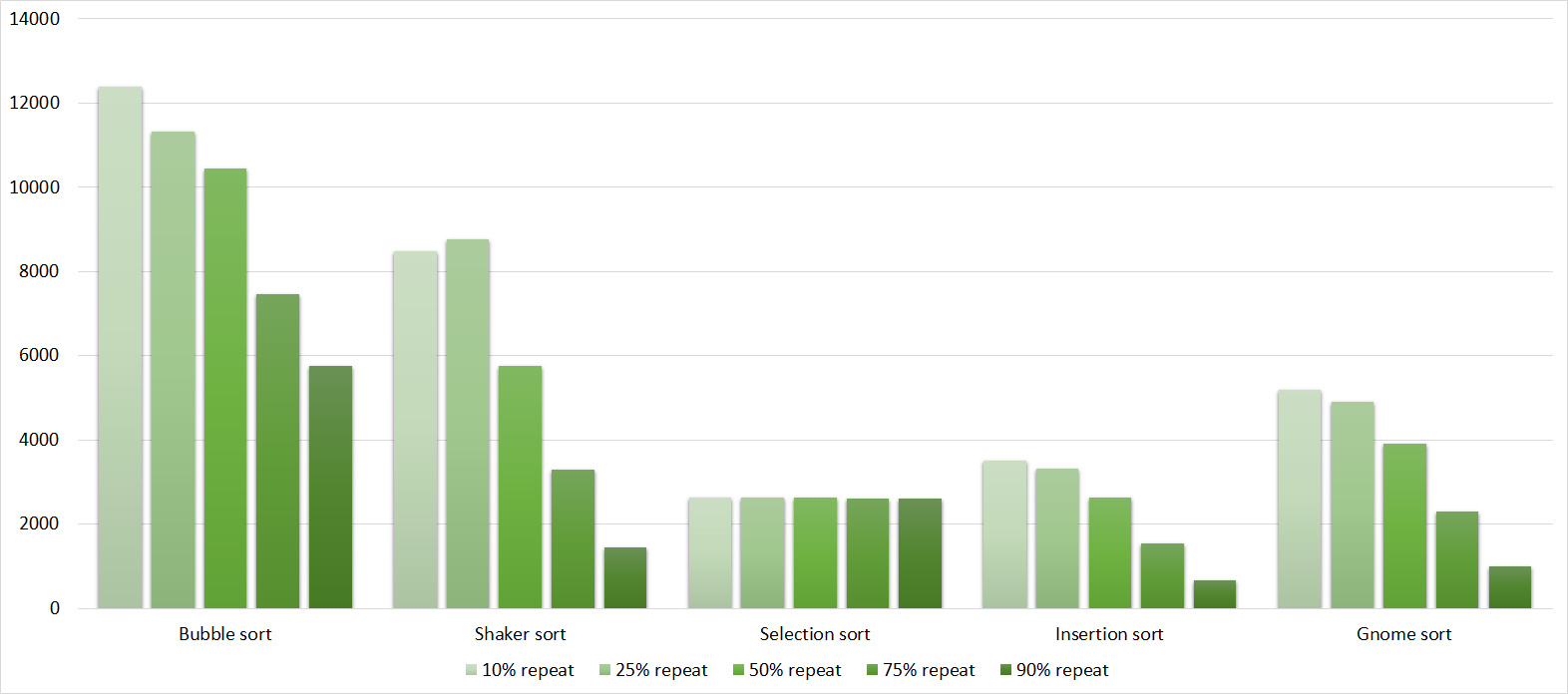
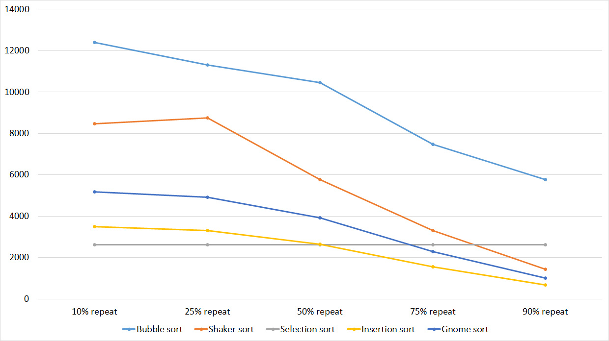
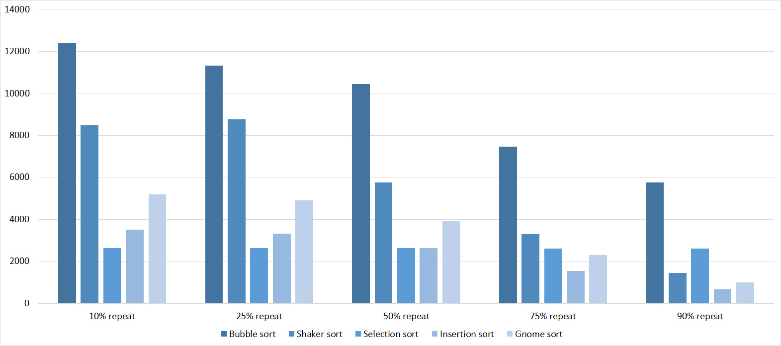
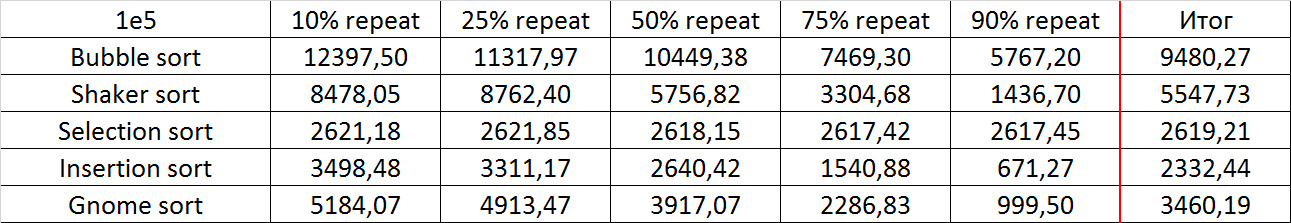
Here, all sortings (except, of course, sorting by choice) worked almost equally, accelerating as the number of repetitions increased.
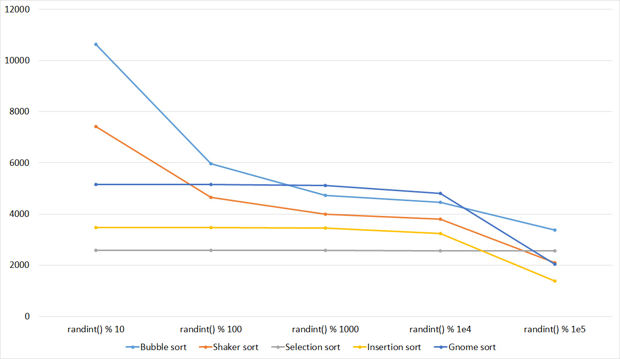
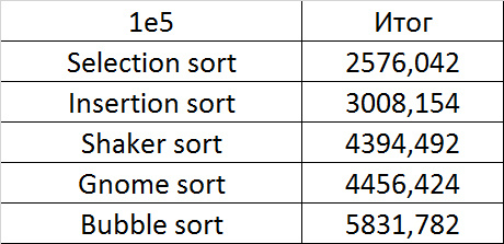
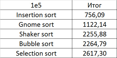
Final results

Due to her absolute indifference to the array, sorting by choice, which worked the fastest on random data, still lost to sorting by inserts. Dwarf sorting turned out to be noticeably worse than the last, which is why its practical use is doubtful. Shaker and bubble sorting turned out to be the slowest.
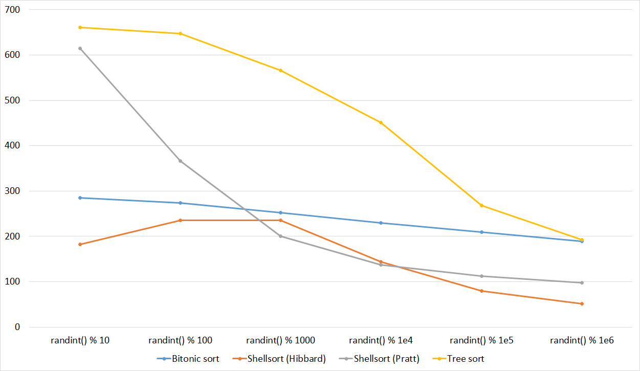
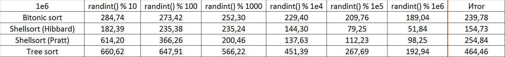
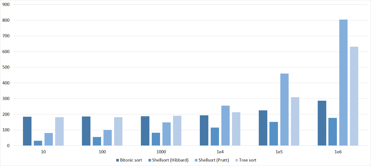
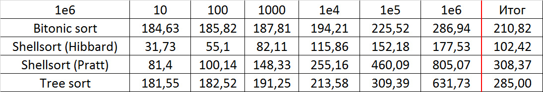
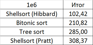
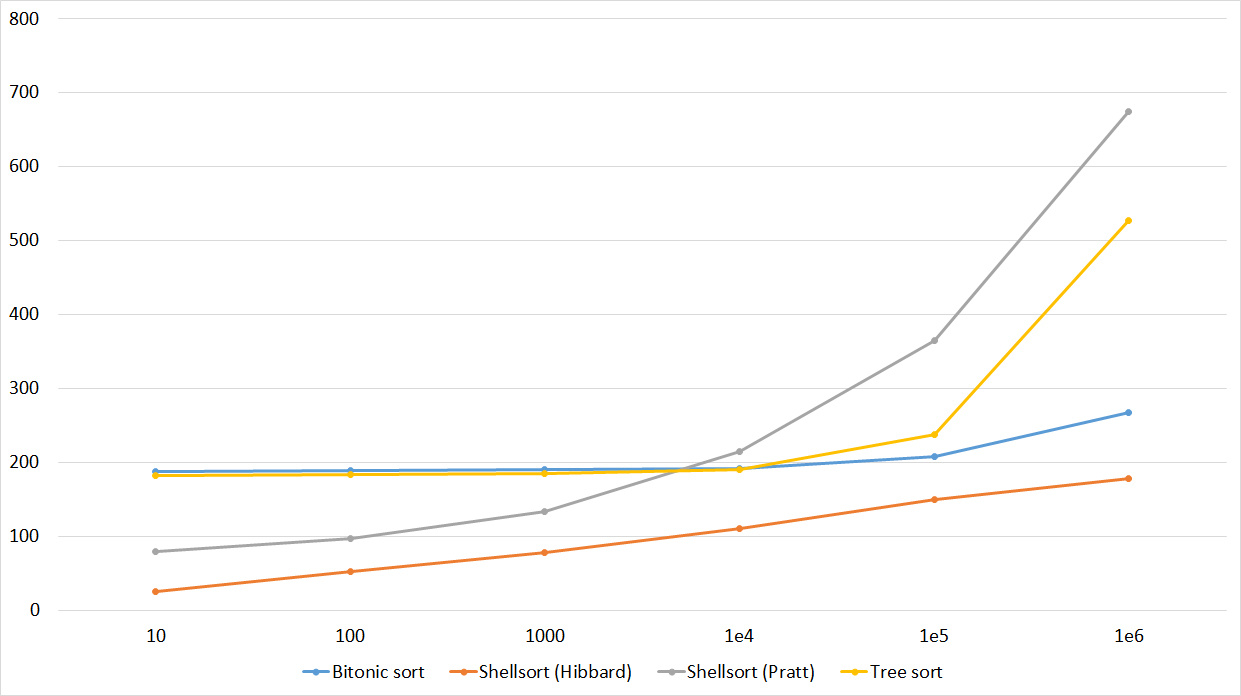
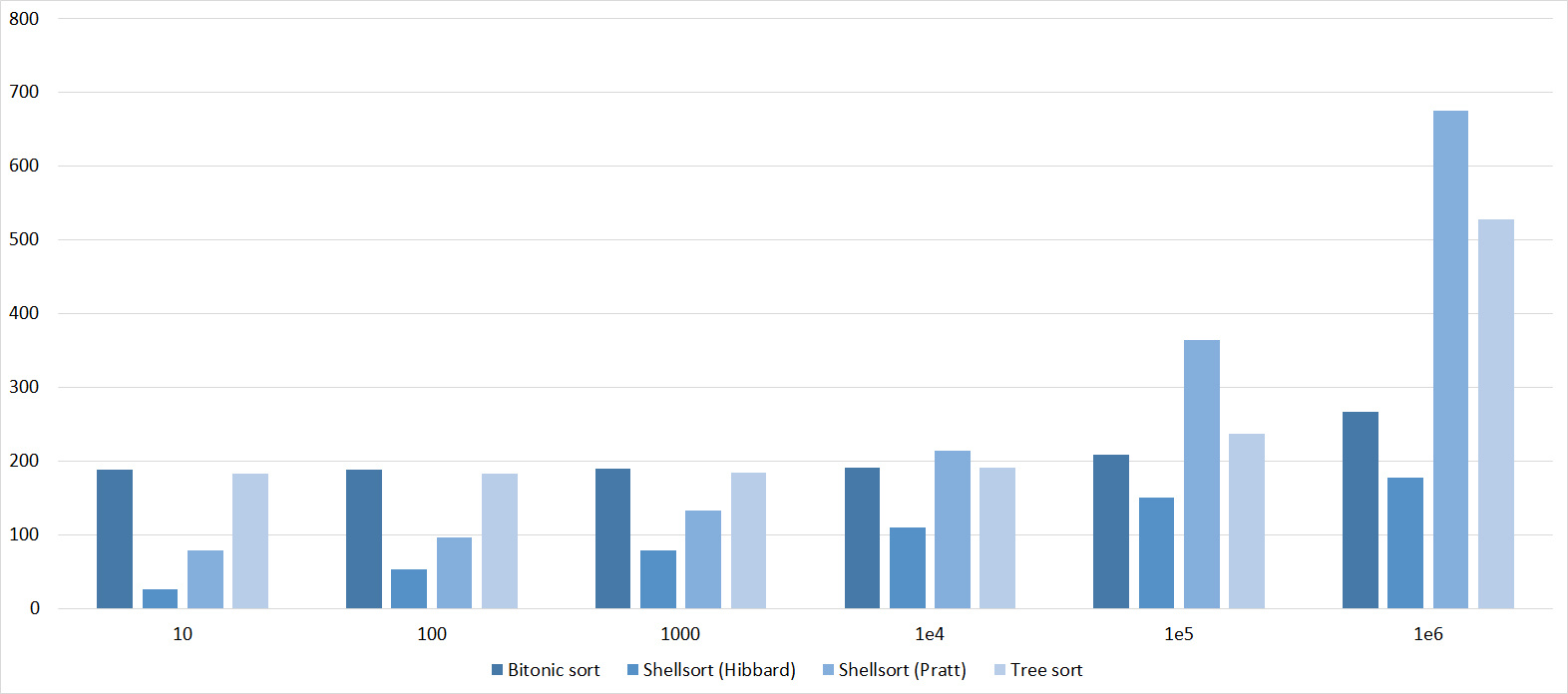
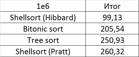
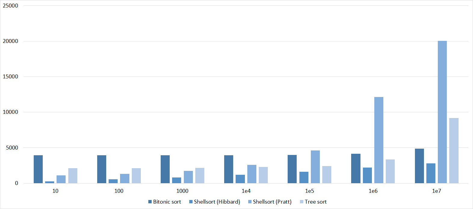
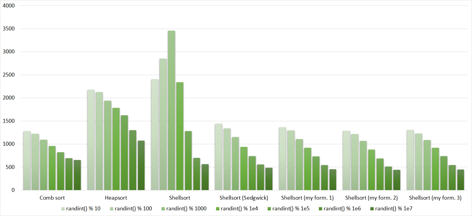
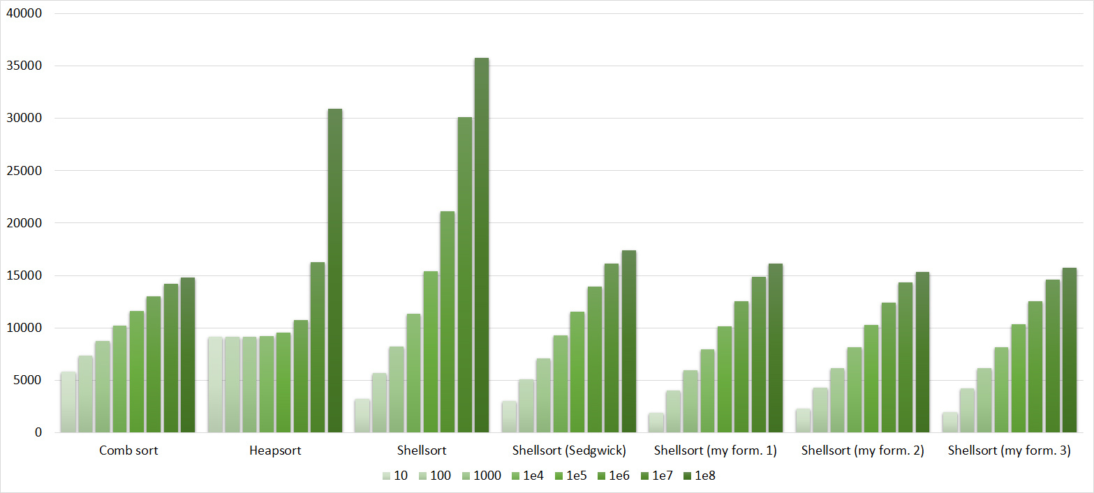
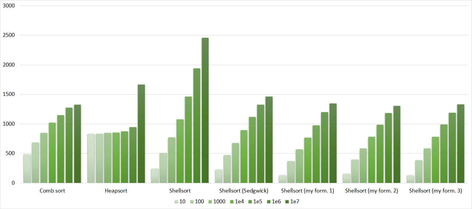
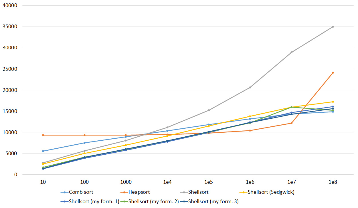
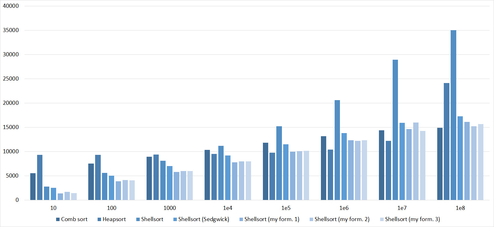
The second group of sorts
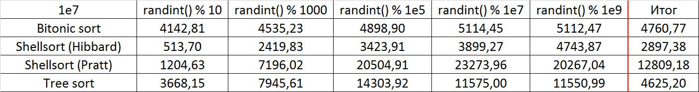
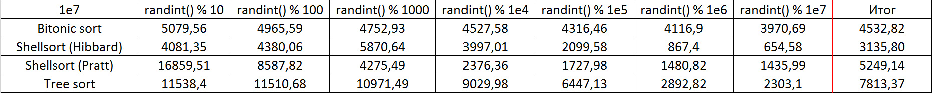
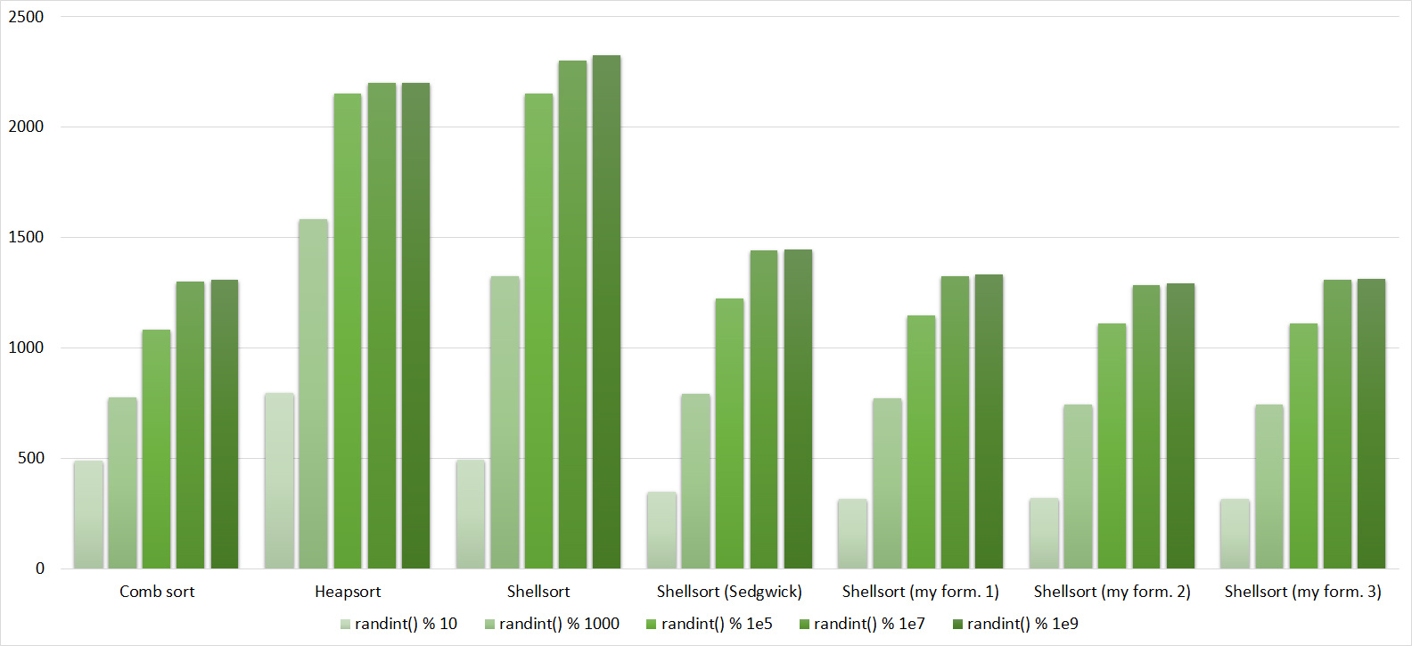
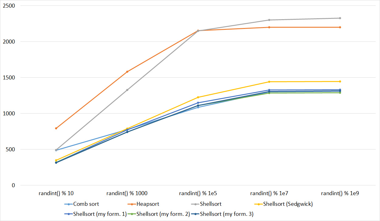
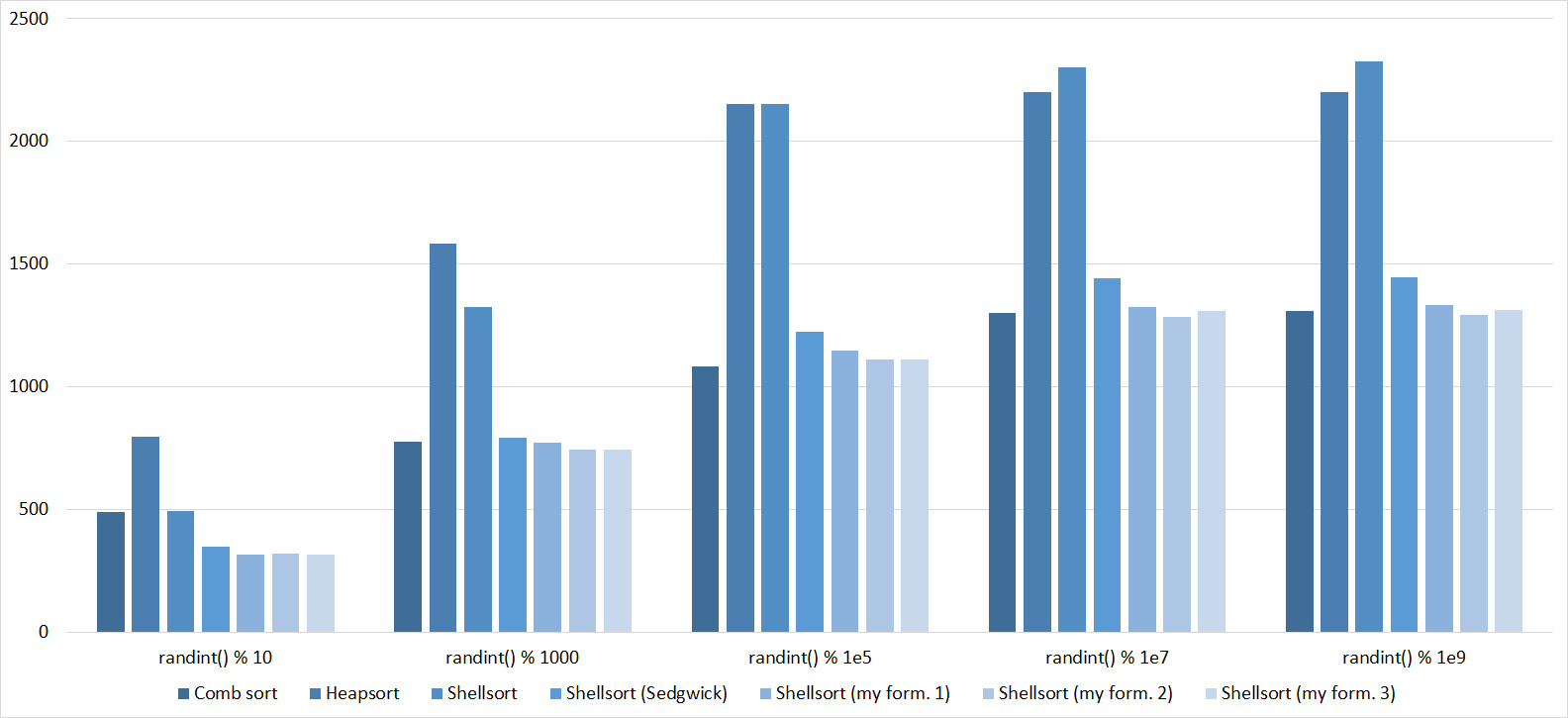
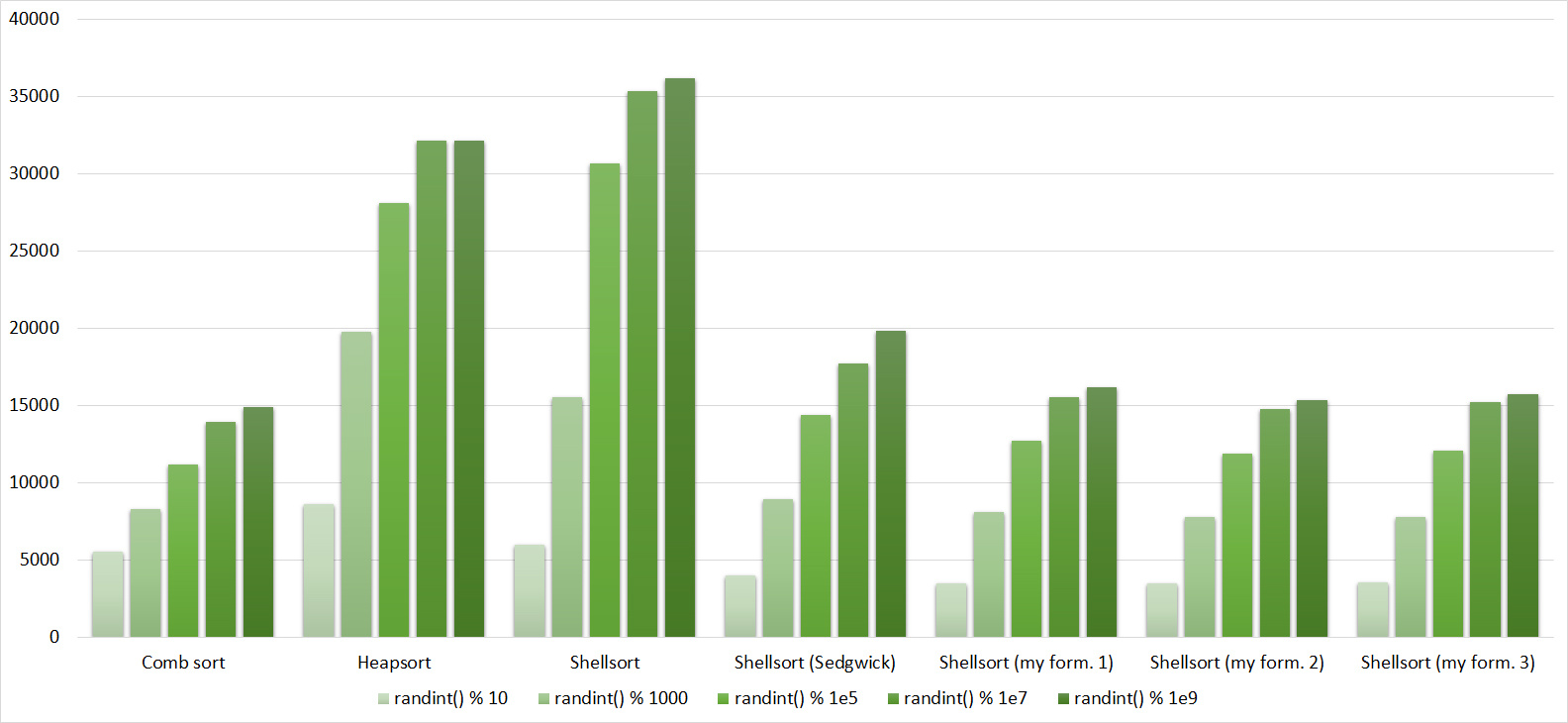
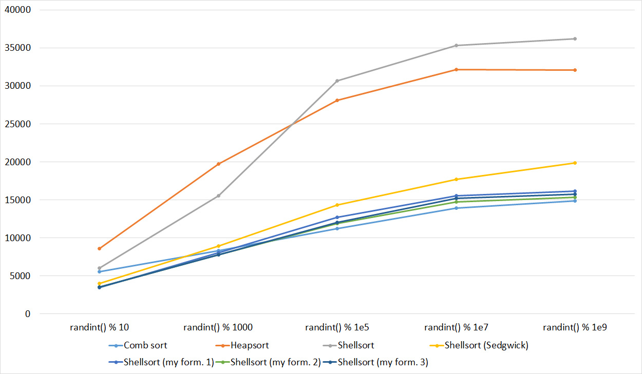
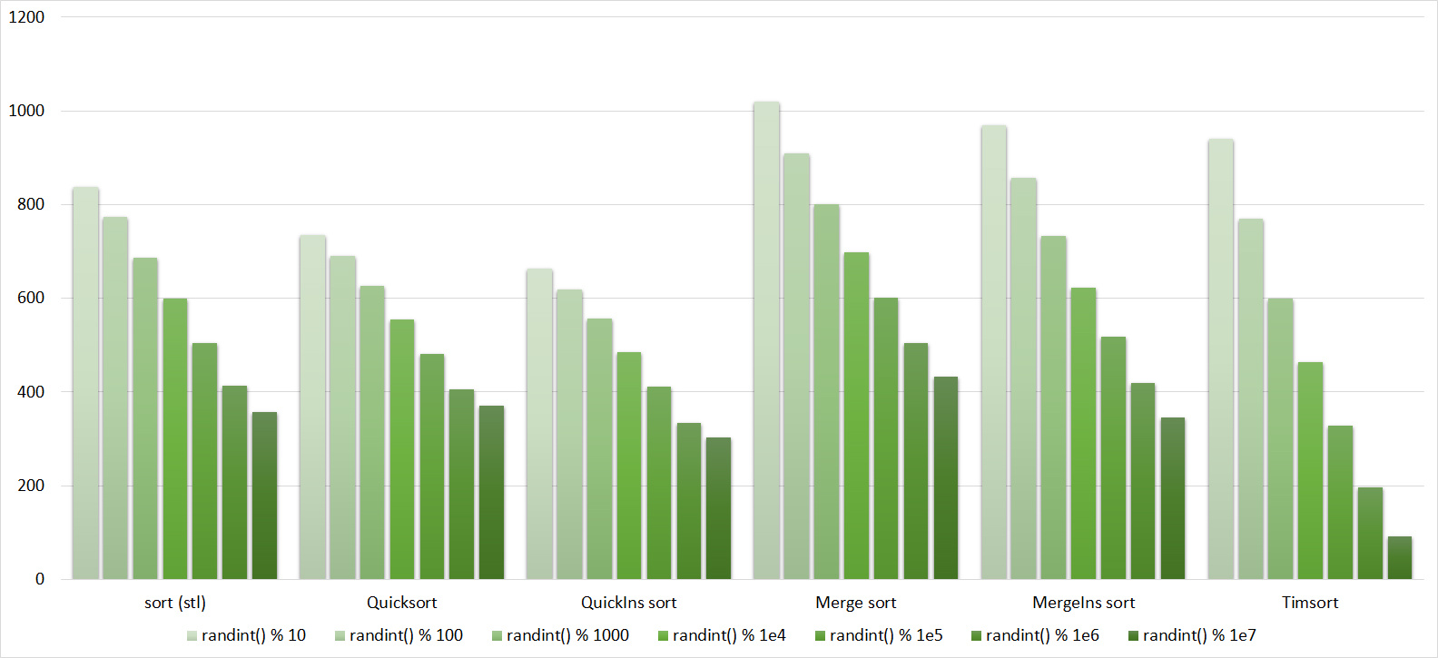
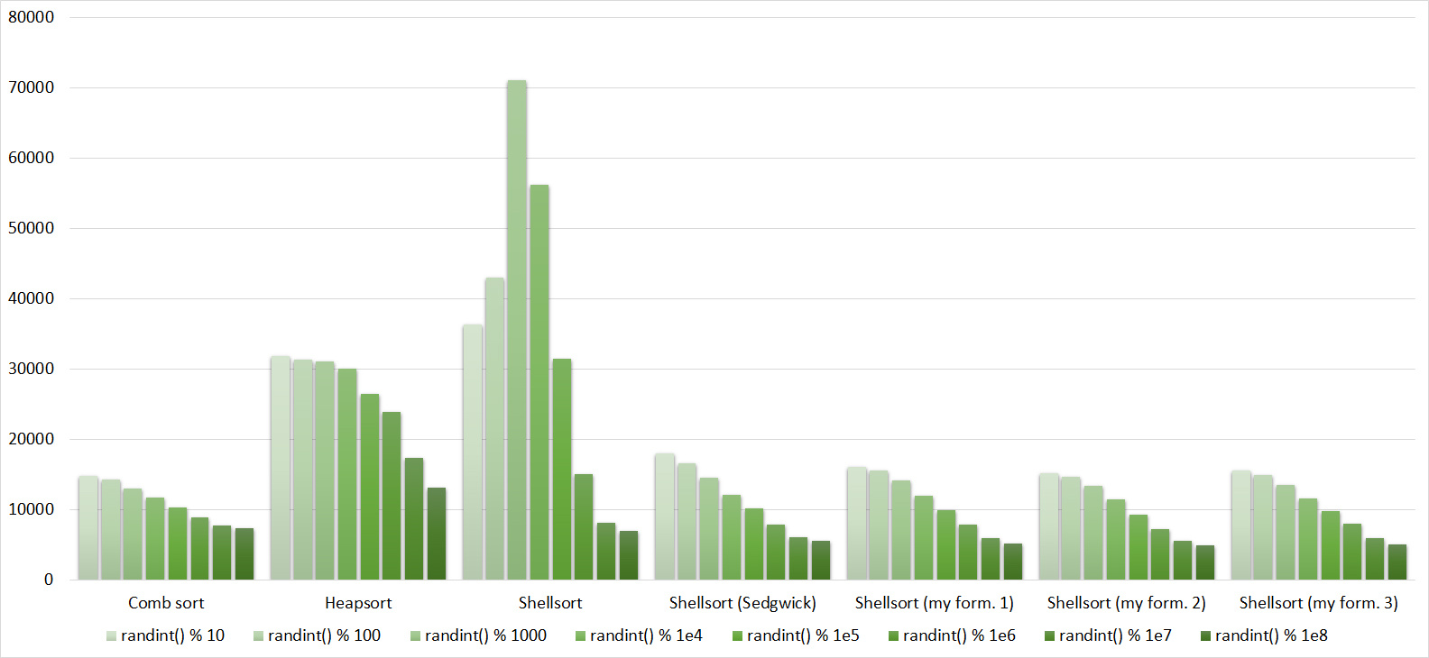
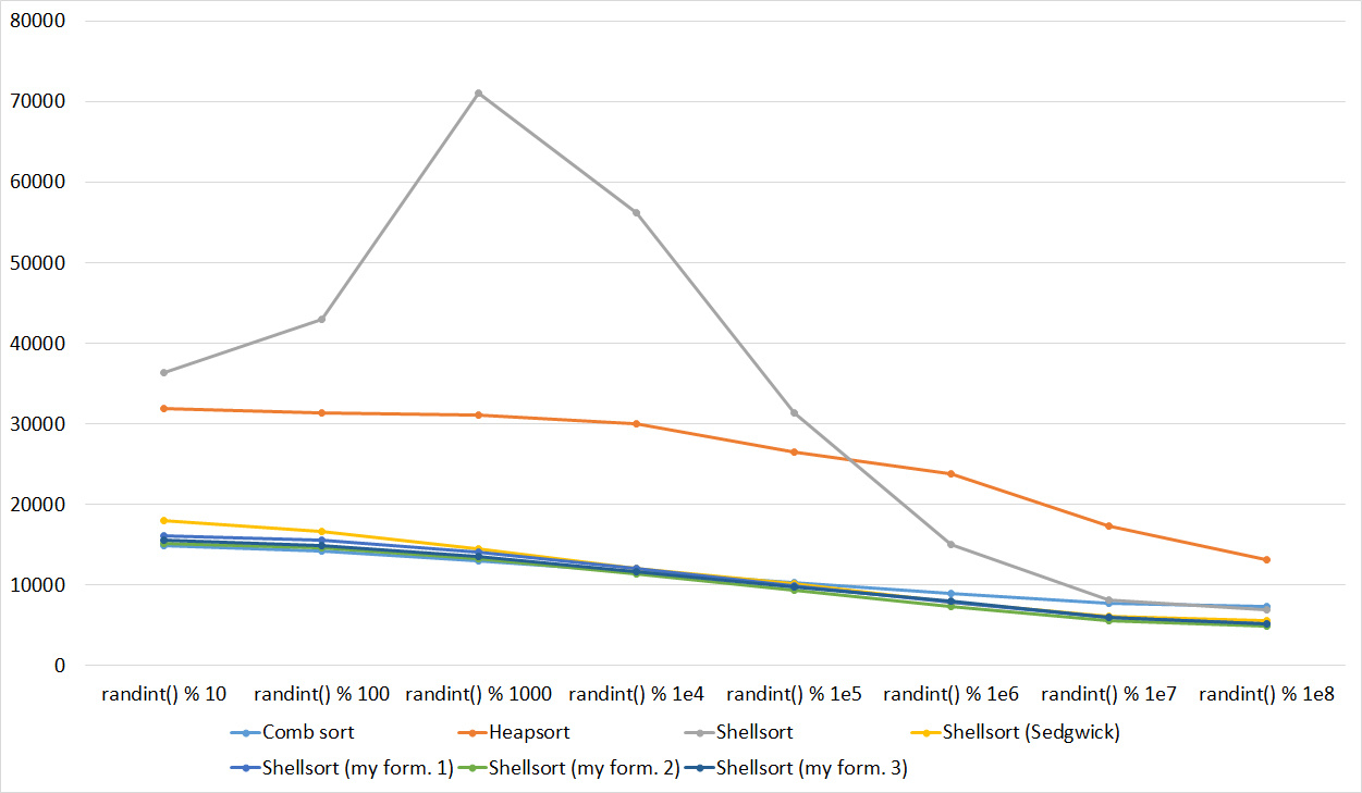
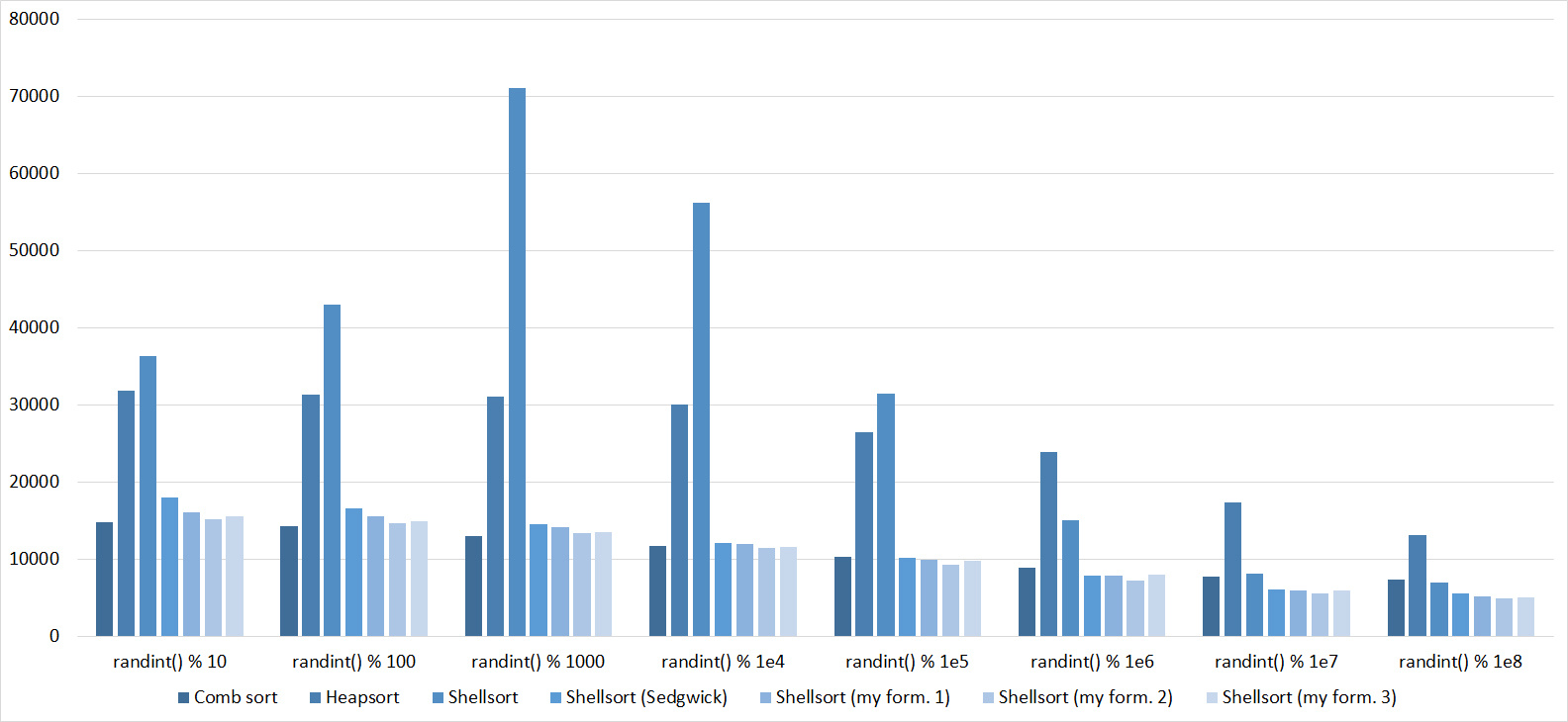
Array of random numbers
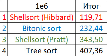
Tables, 1e6 elements
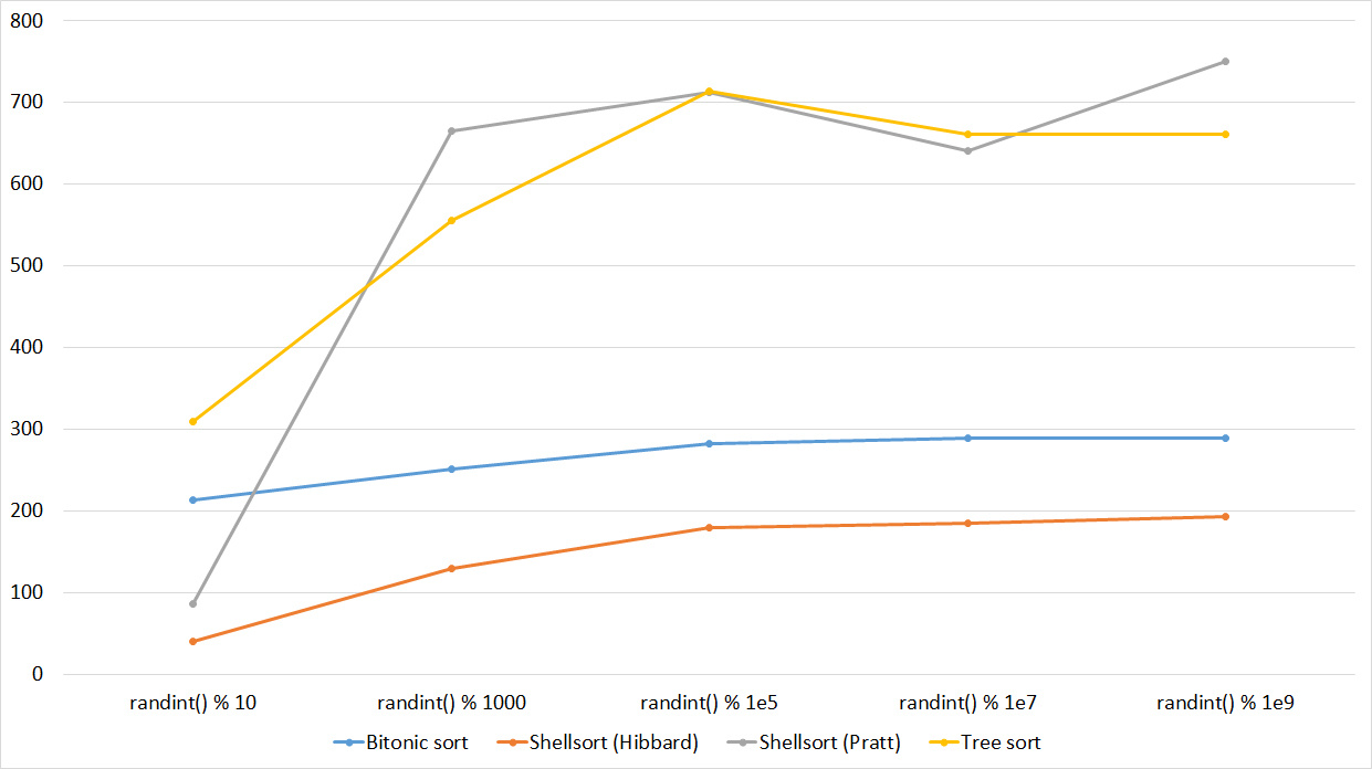
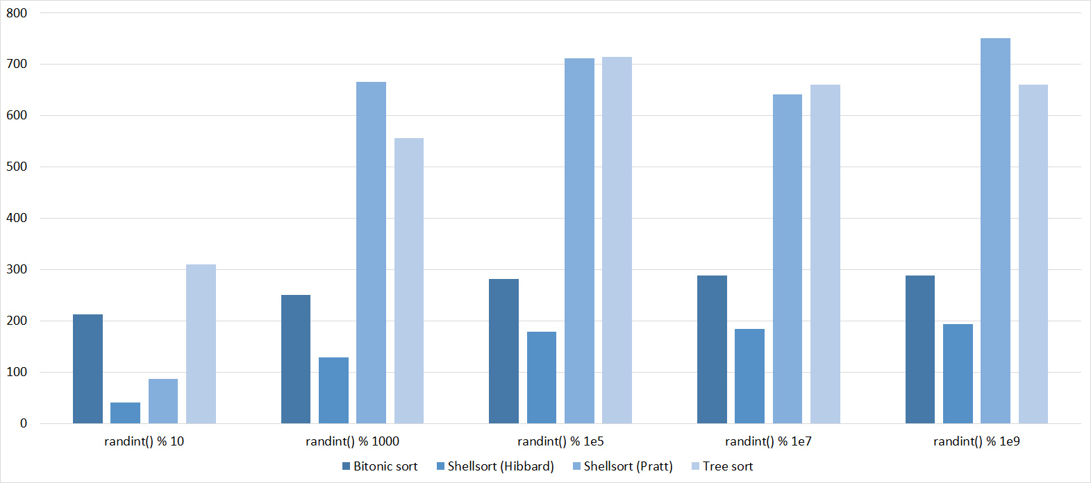


Shell sorting with Pratt's sequence behaves very strange, the rest is less clear. Tree sorting loves partially sorted arrays, but does not like repetition, perhaps, therefore, the worst time of work is in the middle.
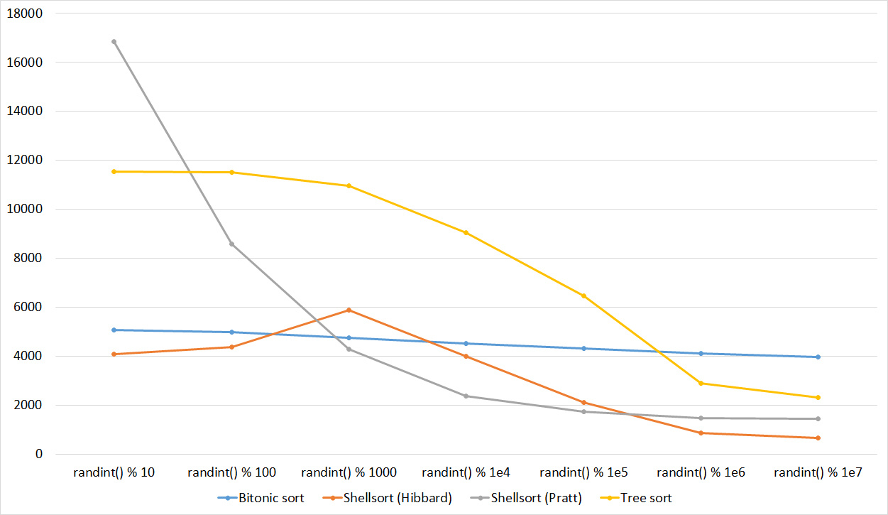
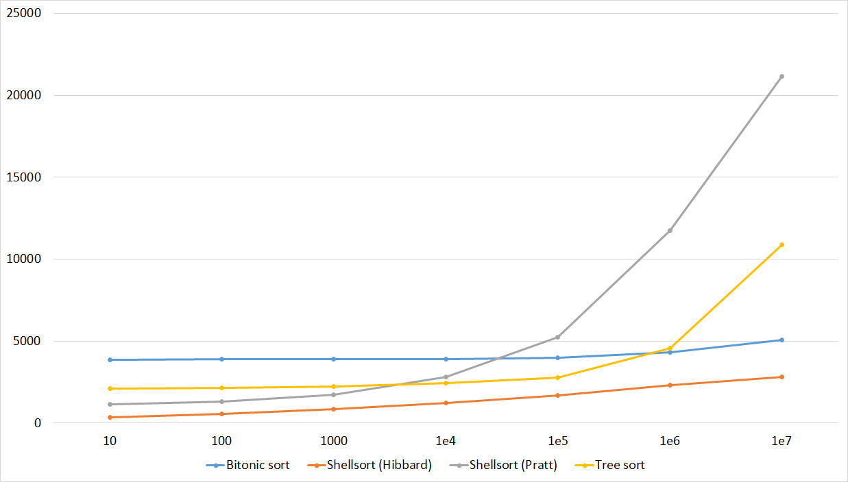
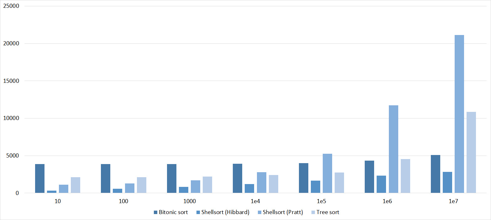
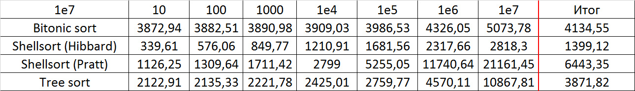
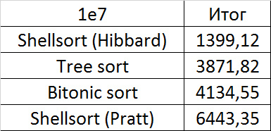
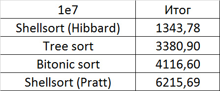
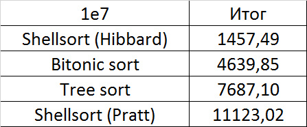
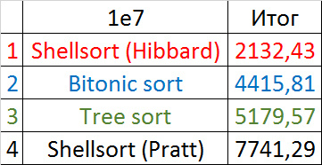
Tables, 1e7 elements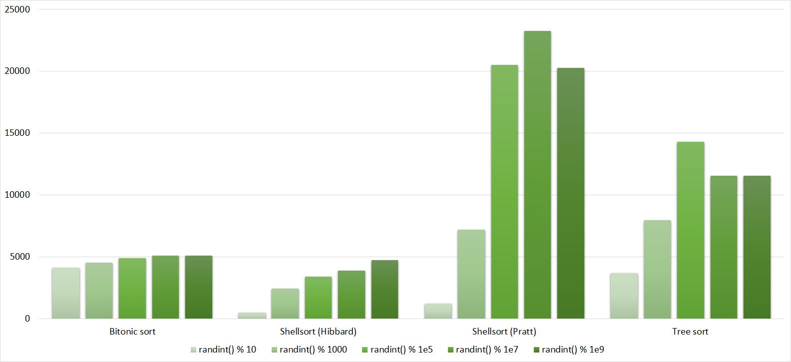
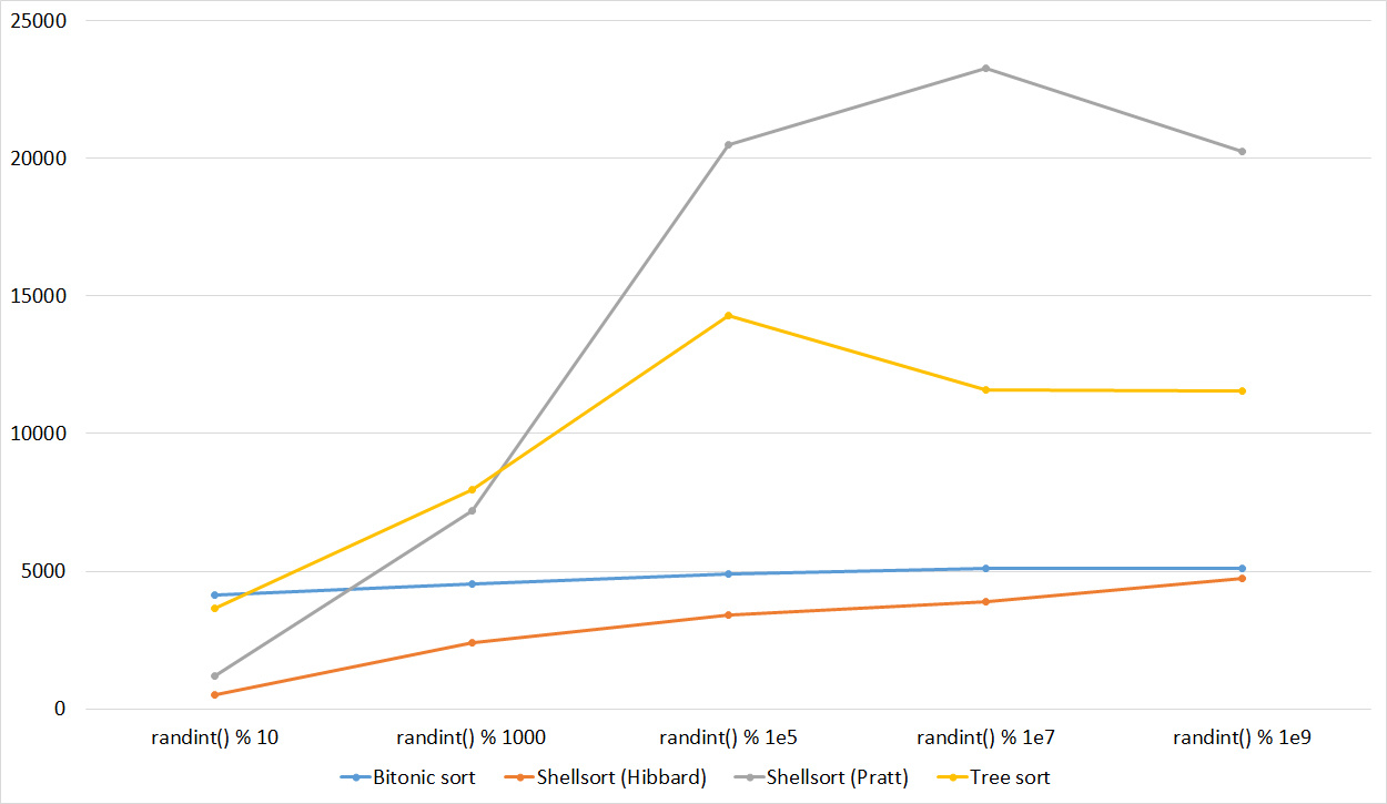
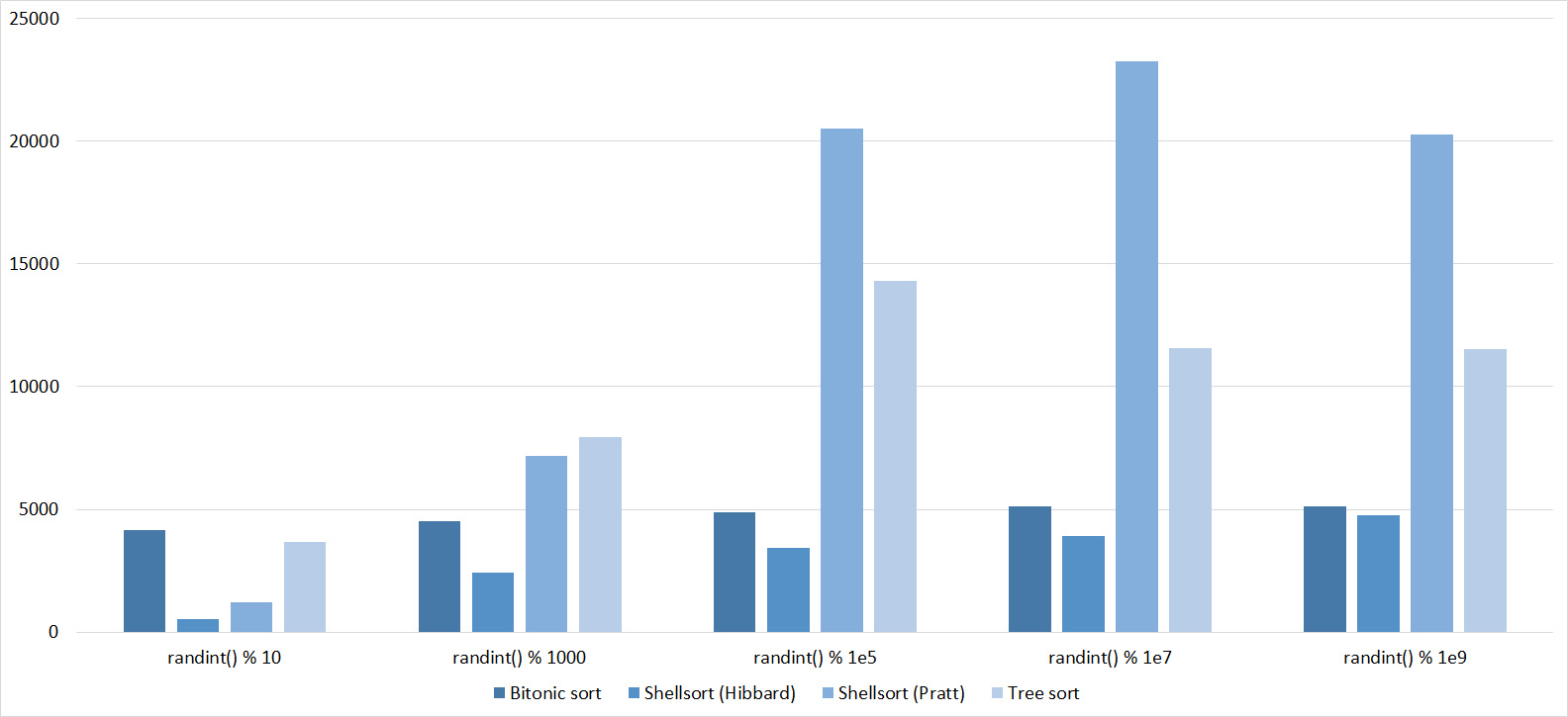
As before, only Shell and Pratt intensified in the second group due to the sorting. The asymptotic effect also becomes noticeable - the tree sorting takes second place, in contrast to the group with a smaller number of elements.
Partially sorted array
Tables, 1e6 elements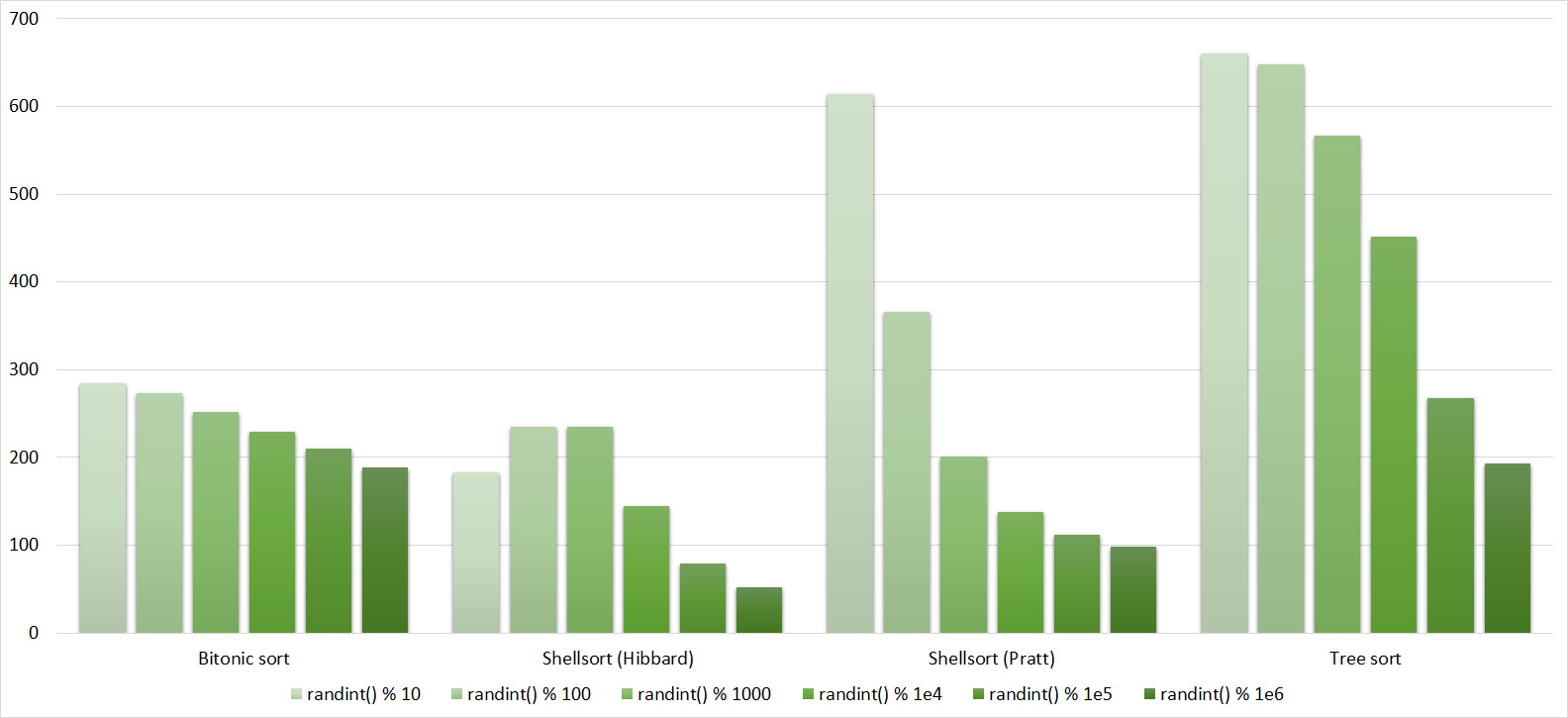


Here all sorts behave in an understandable way, except for Shell and Hibbard, who for some reason does not immediately begin to accelerate.
Tables, 1e7 elements

Here everything is, in general, as before. Even the asymptotic sorting of the tree did not help her to escape from the last place.
Swaps
Tables, 1e6 elements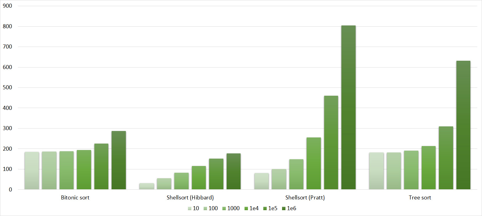
Tables, 1e7 elements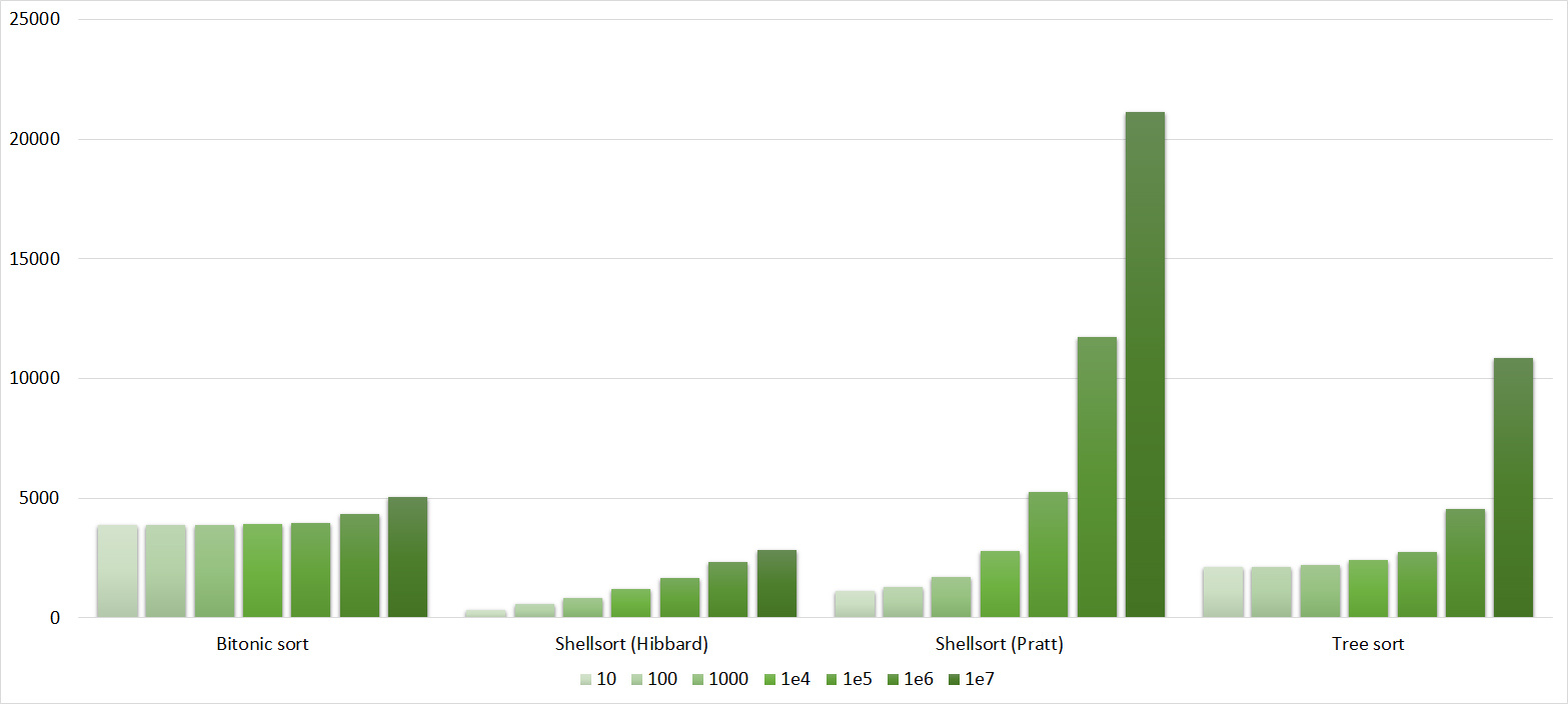
Here it is noticeable that in Shell sorts there is a big dependence on partial sorting, since they behave almost linearly, and the other two only fall strongly on the last groups.
Permutation changes
Tables, 1e6 elements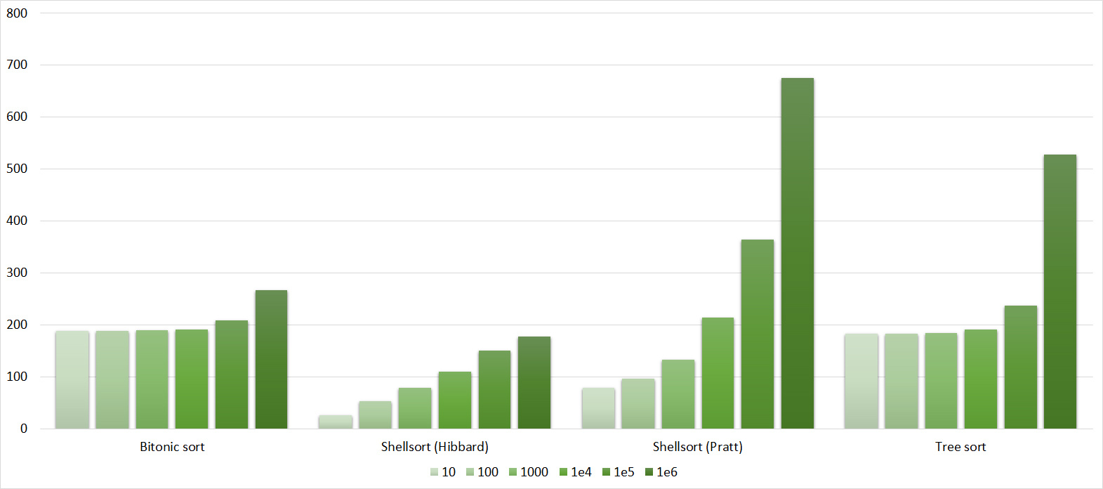

Tables, 1e7 elements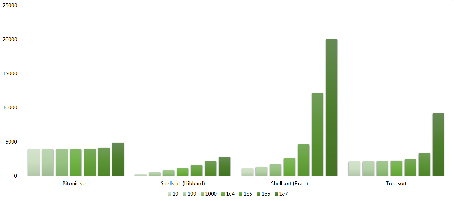


Here everything looks like the previous group.
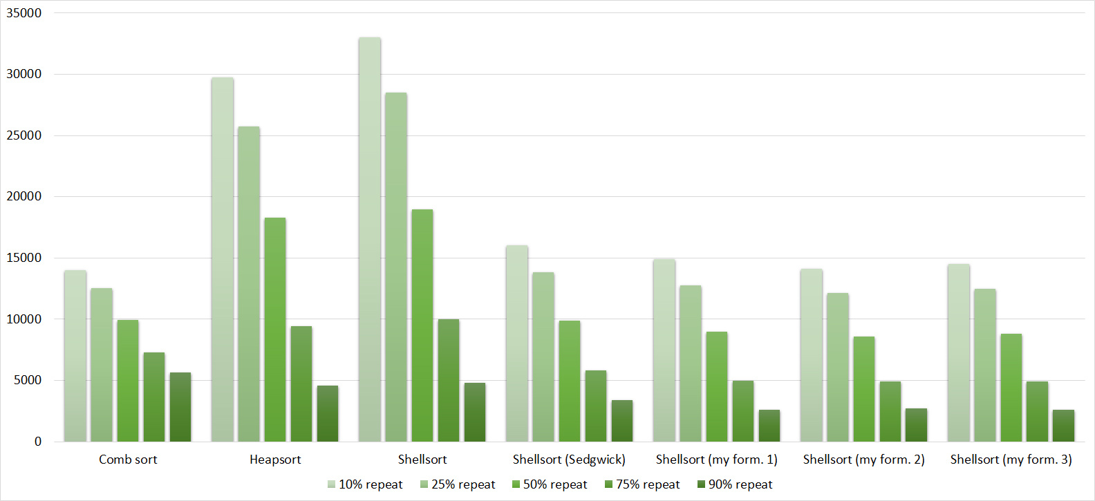
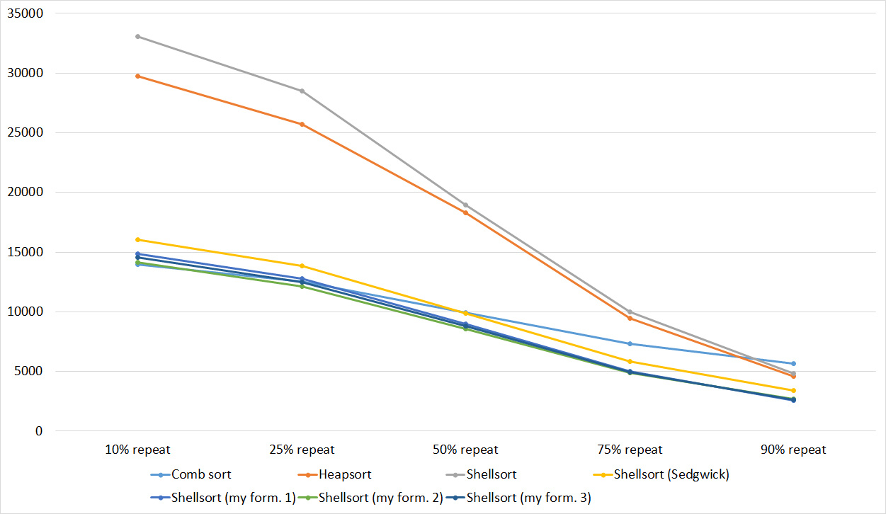
Replays
Tables, 1e6 elements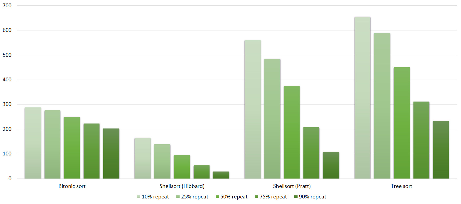
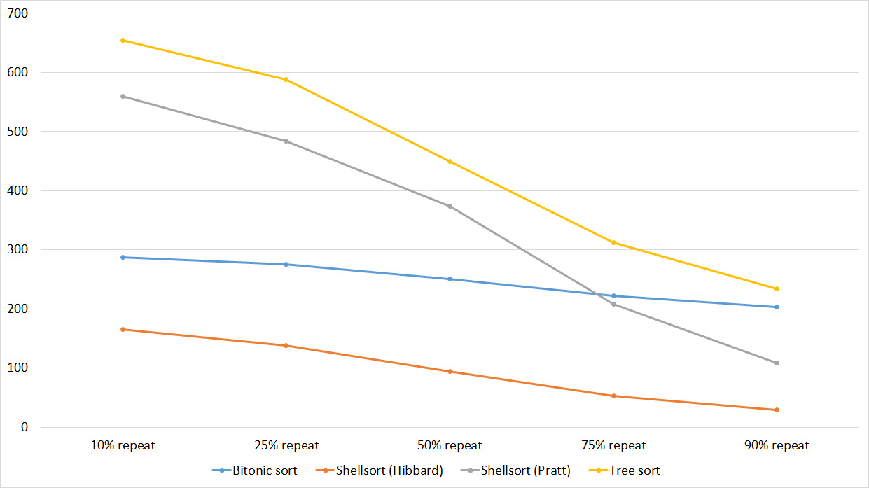


Again, all the sorting showed an amazing balance, even biton, which, it would seem, almost does not depend on the array.
Tables, 1e7 elements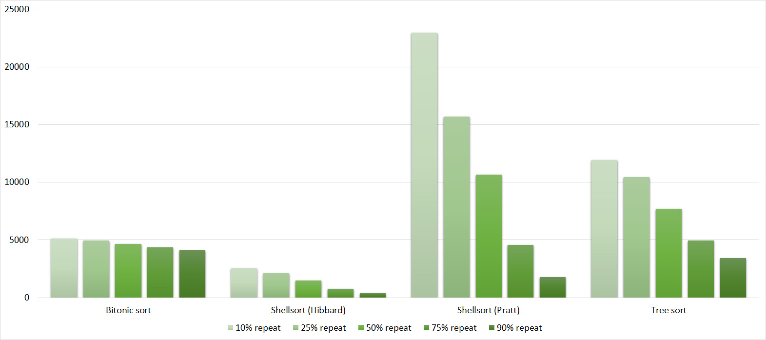
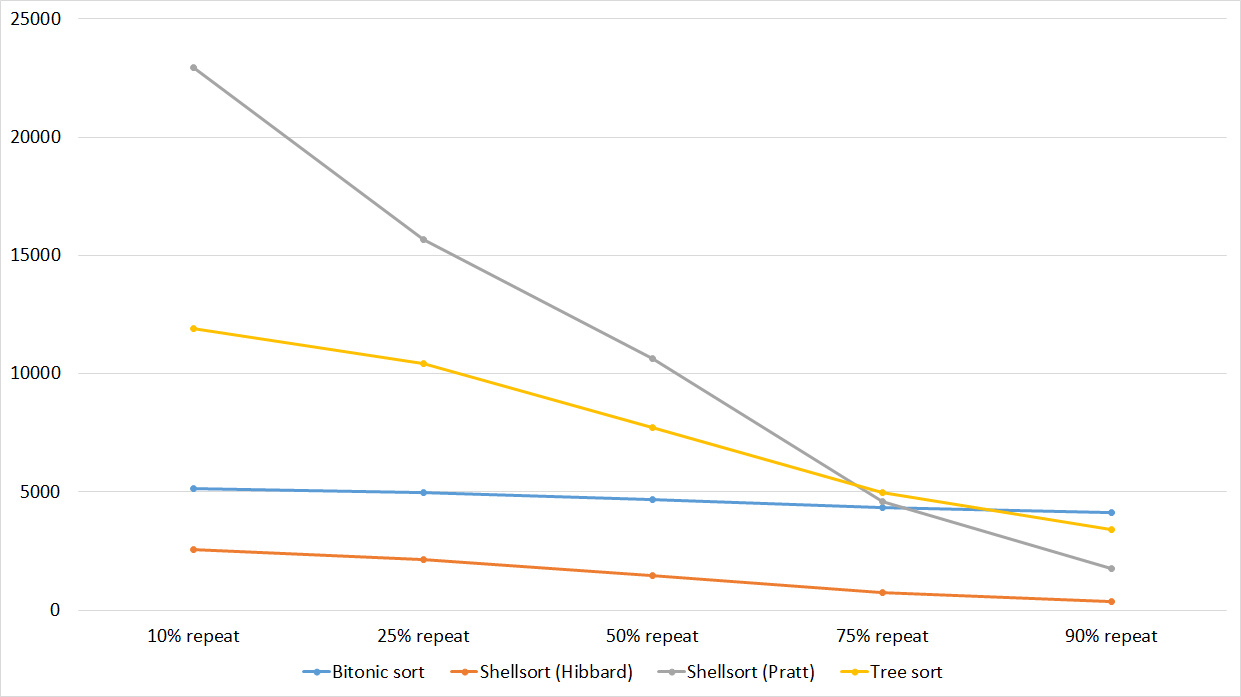
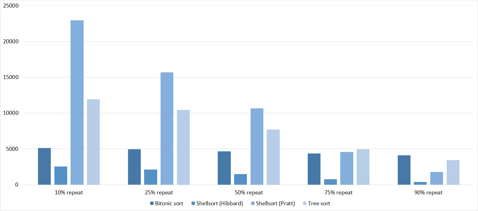

Nothing interesting.
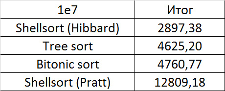
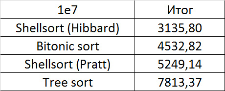
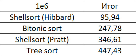
Final results
Convincing first place was taken by the sorting of Shell by Hibbard, not losing in any intermediate group. It might have been worth sending it to the first group of sorts, but ... it is too weak for this, and even then almost no one would be in the group. Biton sorting pretty confidently took second place. The third place with a million elements was taken by another sort of Shell, and at ten millions by sorting by a tree (asymptotics was affected). It is worth noting that with a tenfold increase in the size of the input data, all the algorithms, except for wood sorting, slowed down almost 20 times, and the latter is only 13.
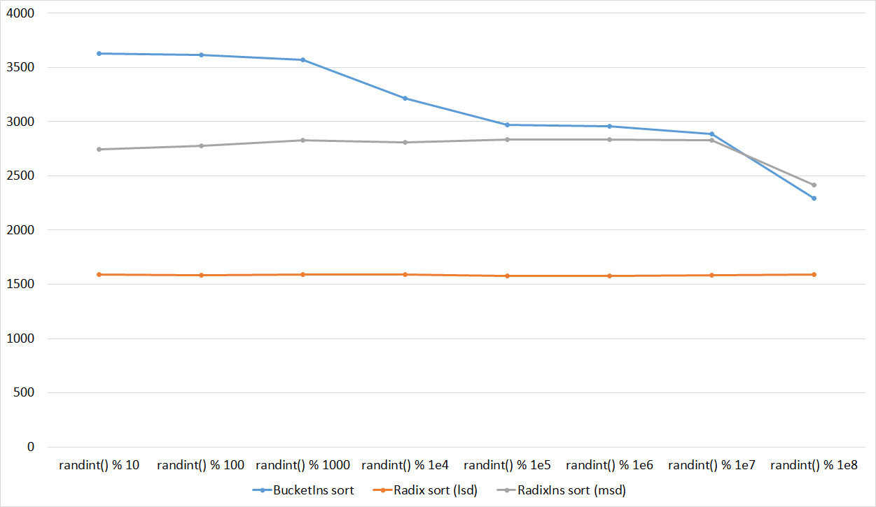
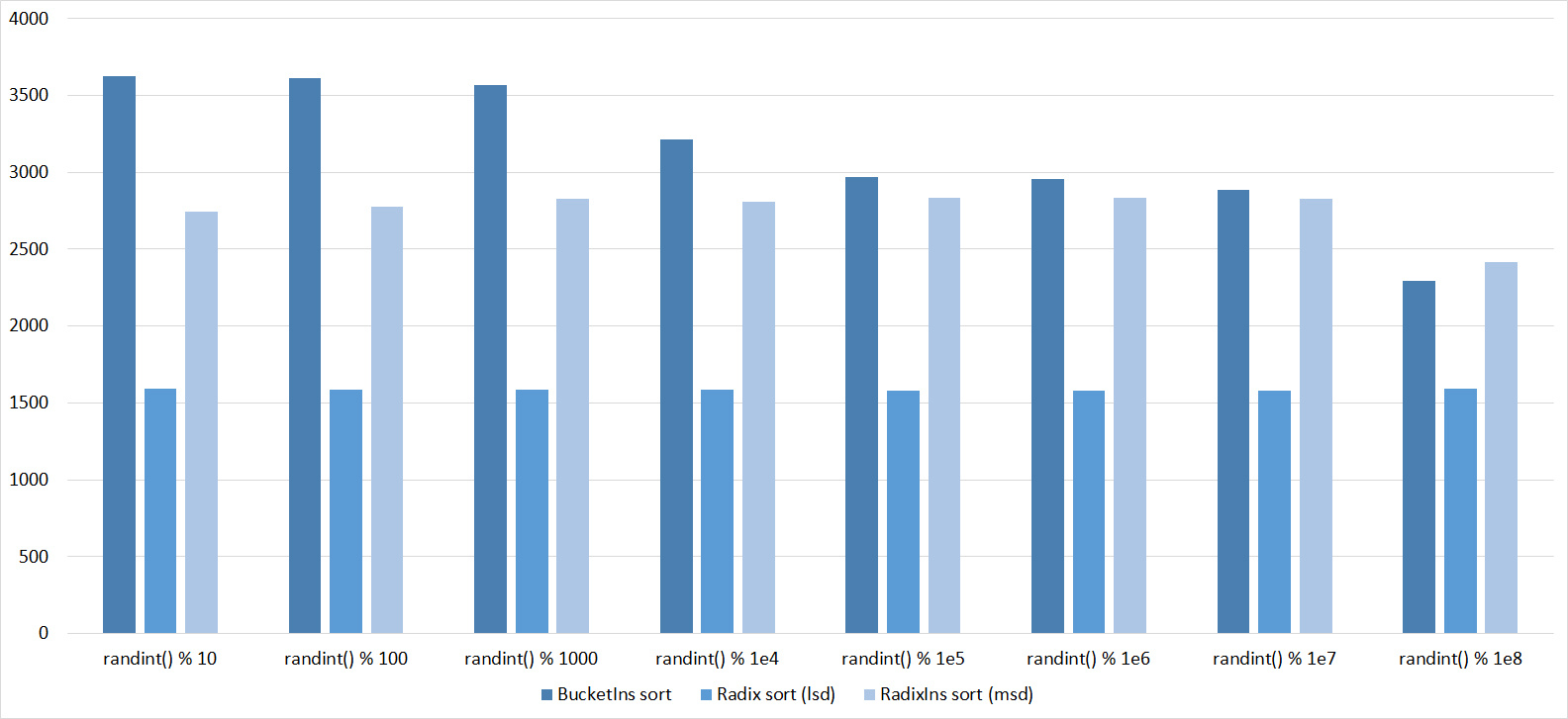
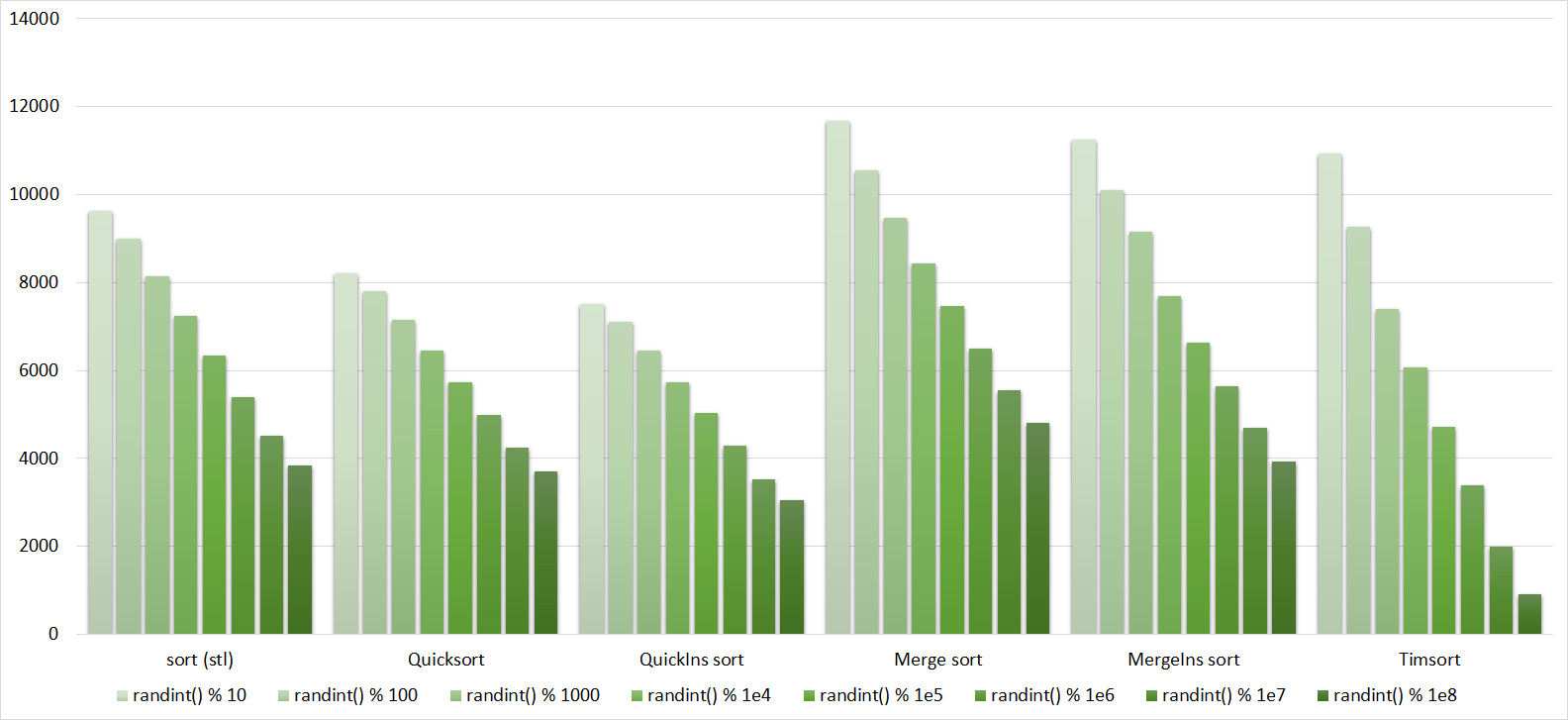
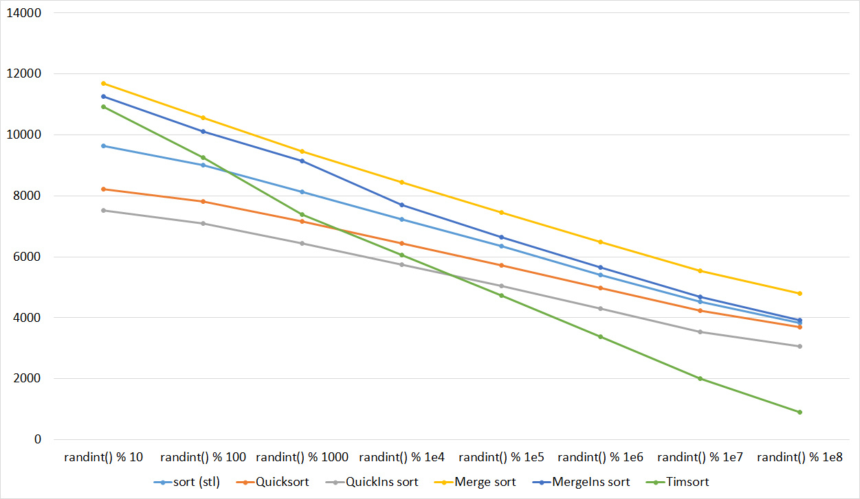
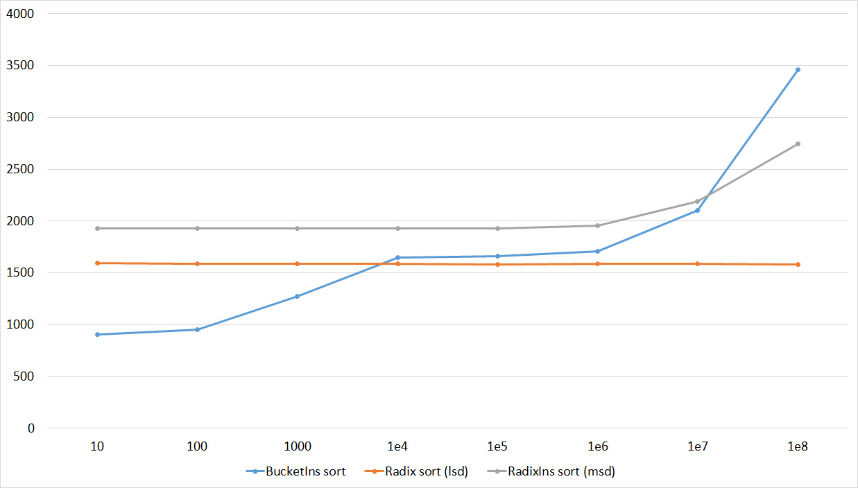
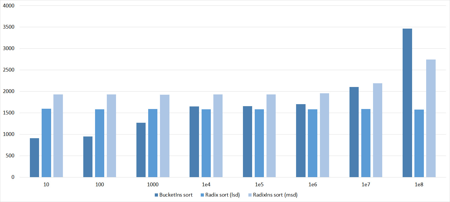
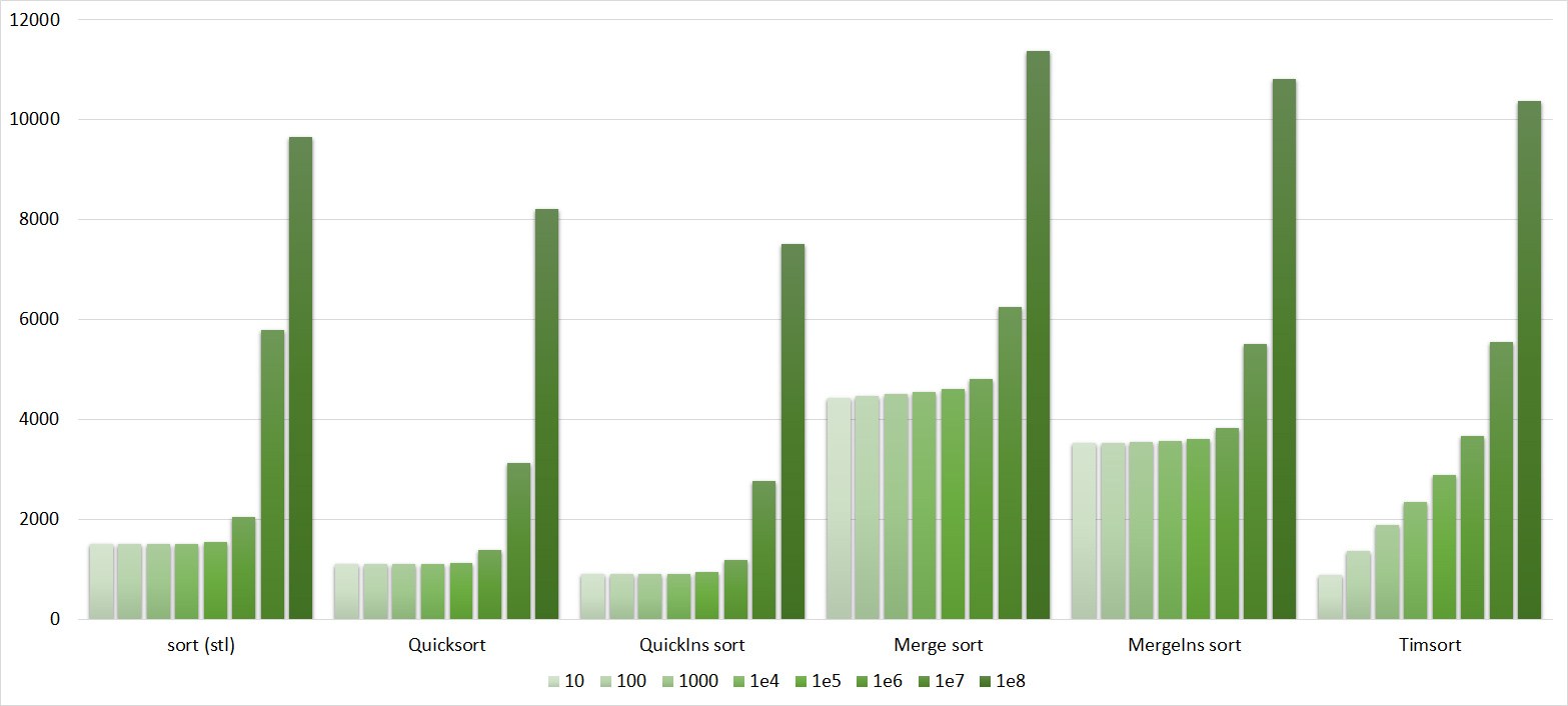
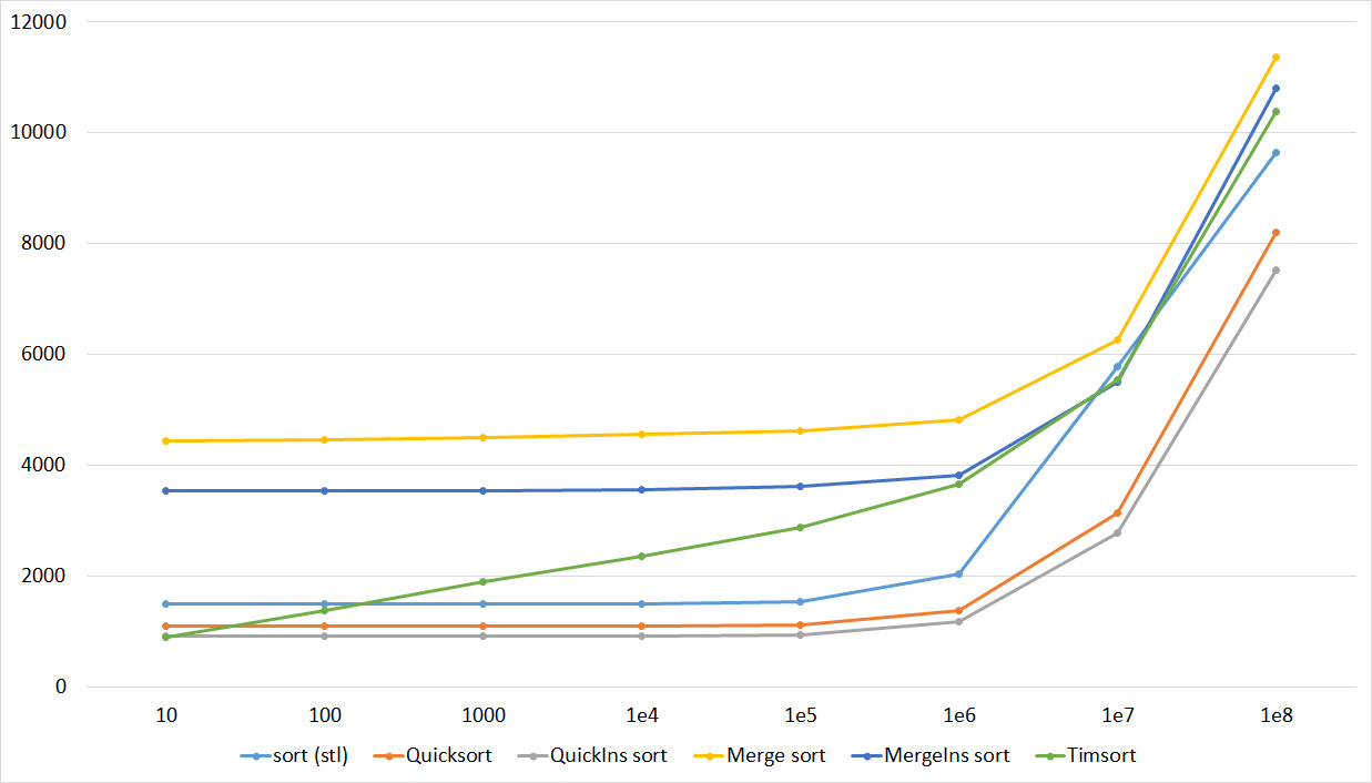
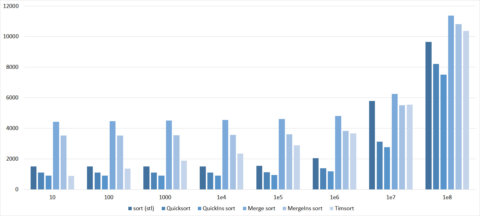
The third group of sorts
, 17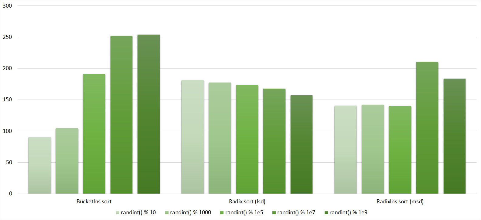

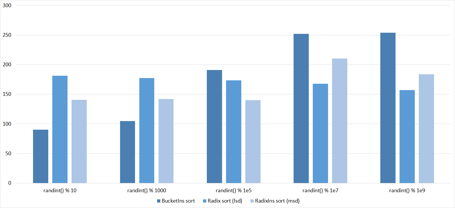
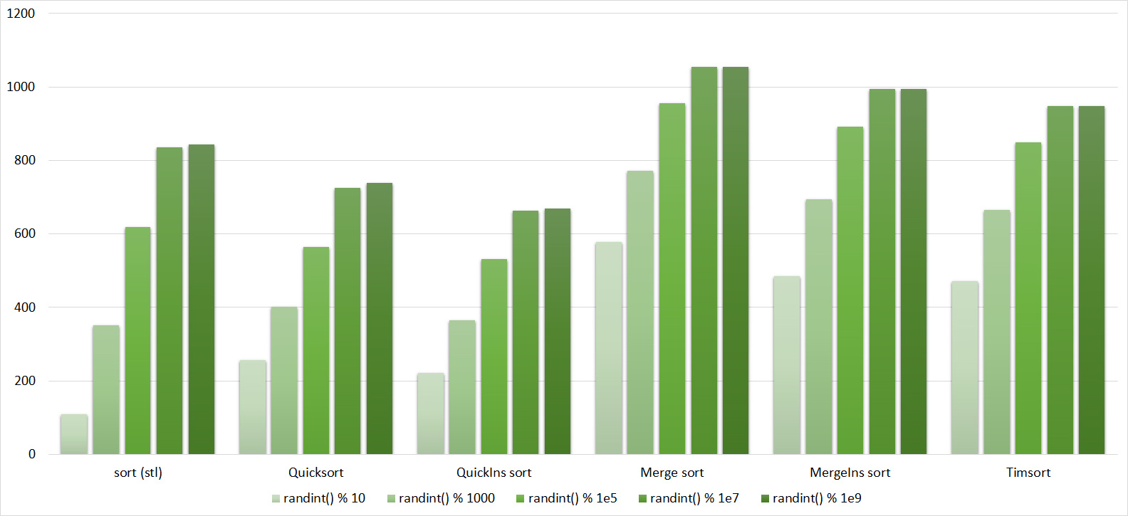
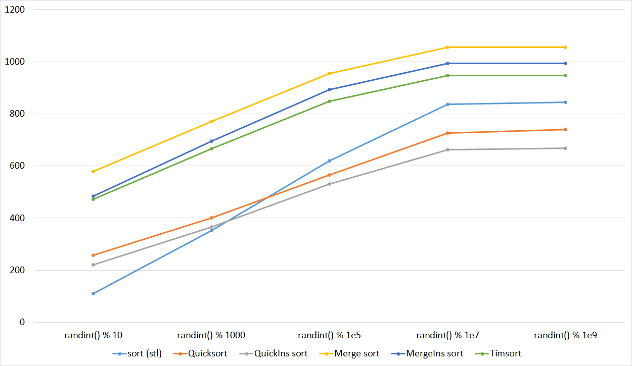
, 18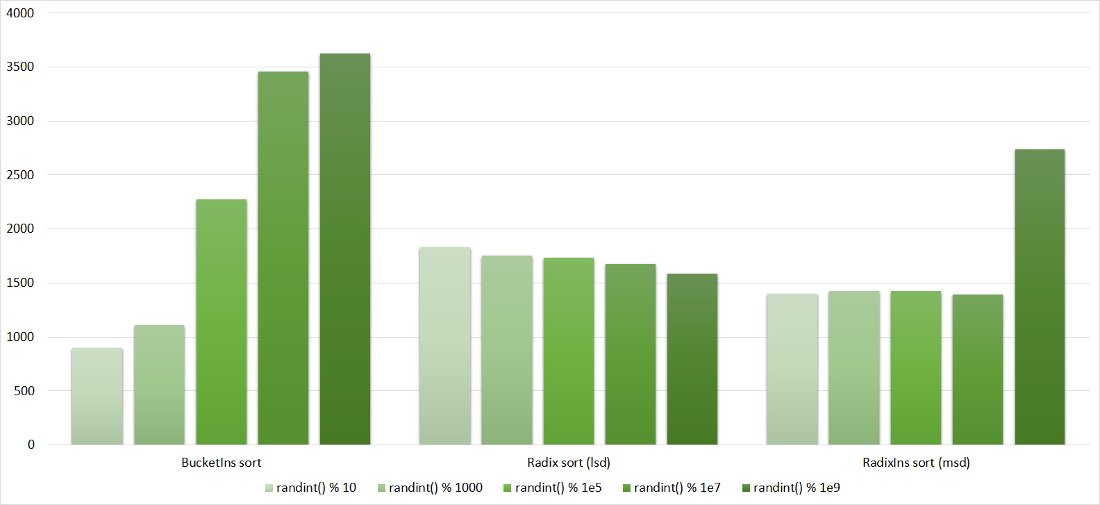


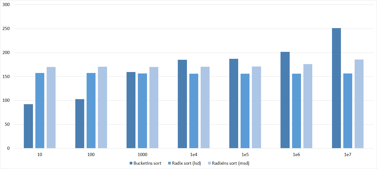
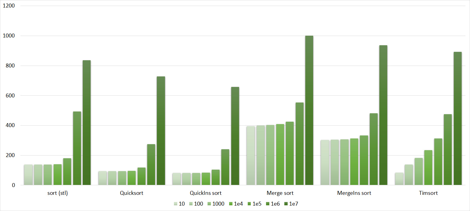
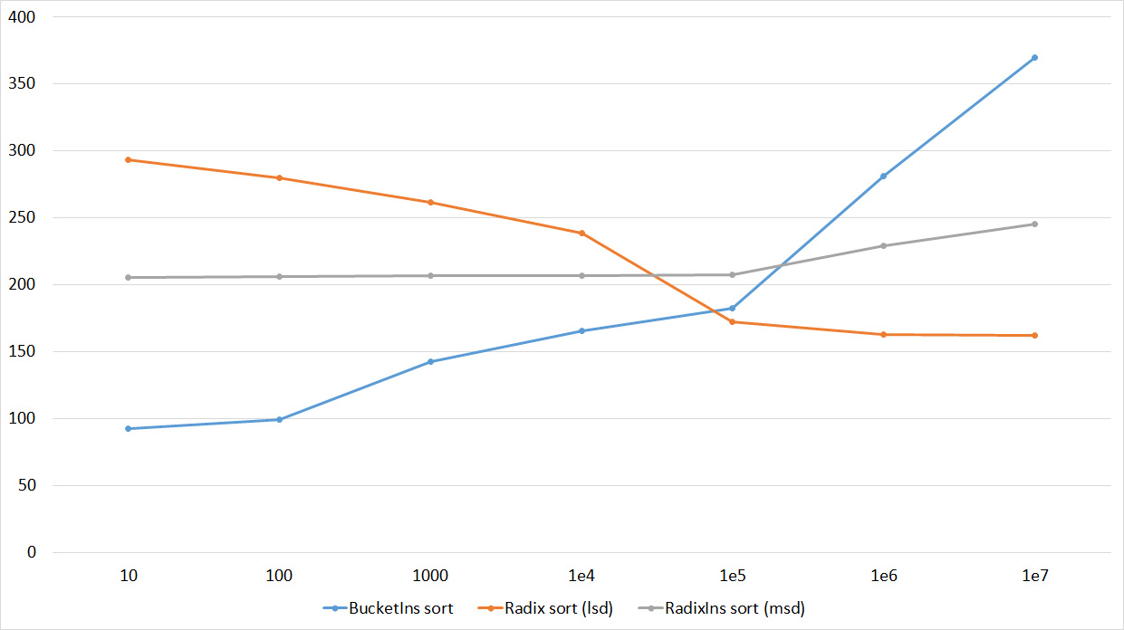
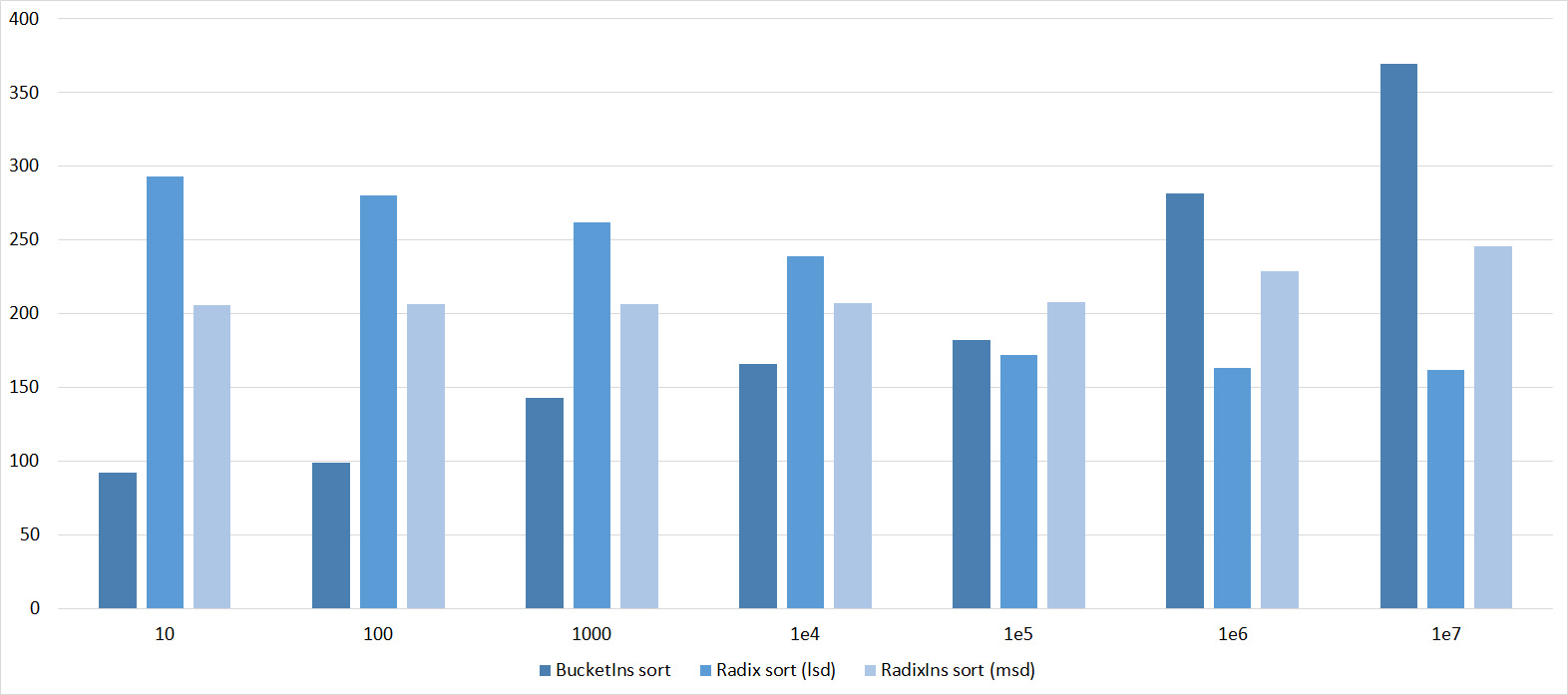
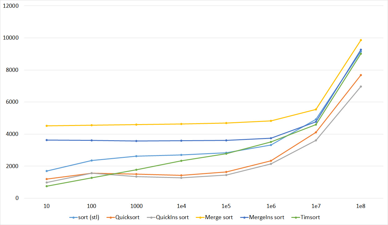
Almost all sorts of this group have almost the same dynamics. Why is almost all sorting accelerated when the array is partially sorted? Exchange sorts work faster because fewer exchanges are needed; in Shell sorting, sorting is performed by inserts, which is greatly accelerated on such arrays; in pyramid sorting, insertion of elements immediately completes screening; in merge sorting, at least half the number of comparisons is performed. Block sorting works the better, the smaller the difference between the minimum and maximum element. Fundamentally different only bitwise sorting, which all this does not matter. The LSD version works the better, the larger the module. The dynamics of the MSD version is not clear to me, that it worked faster than LSD was surprised.
Partially sorted array
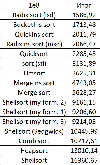
Tables, 1e7 elements


Tables, 1e8 elements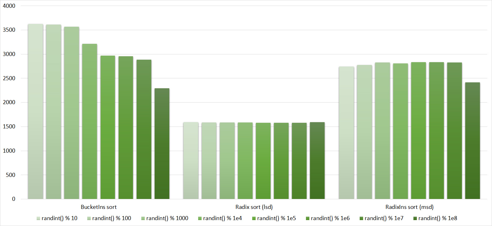

Everything is pretty clear here too. The Timsort algorithm has become noticeable, the sorting affects it more strongly than the others. This allowed this algorithm to almost equal the optimized version of quick sort. Block sorting, despite the improvement in working time with partial sorting, could not overtake the bitwise sorting.
Swaps
Tables, 1e7 elements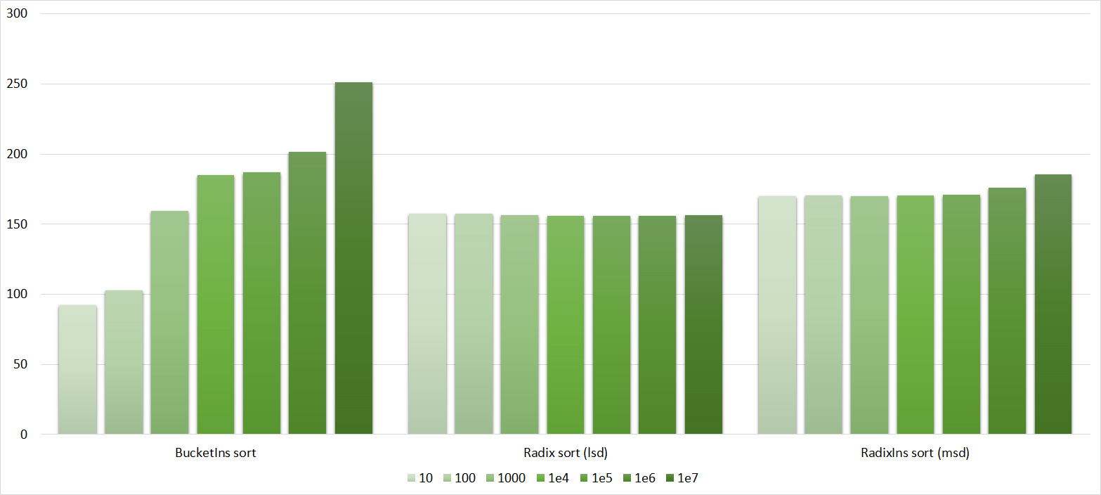


Tables, 1e8 elements

Quick sorts worked very well here. This is most likely due to the successful selection of the support element. Everything else is almost the same as in the previous group.
Permutation changes
Tables, 1e7 elements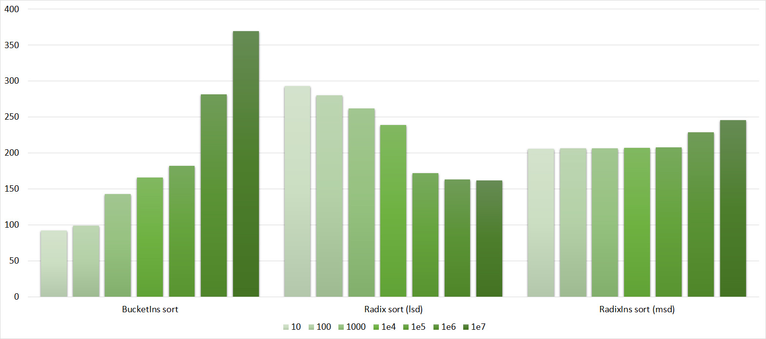


Tables, 1e8 elements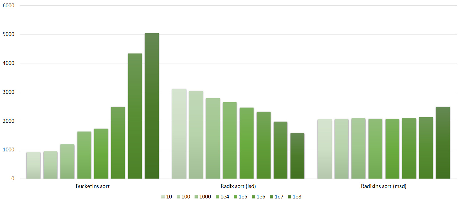


I managed to achieve the desired goal - the bitwise sorting fell even below the adapted quick. Block sorting was better than the rest. For some reason, timsort overtook the built-in sorting of C ++, although it was lower in the previous group.
Replays
Tables, 1e7 elements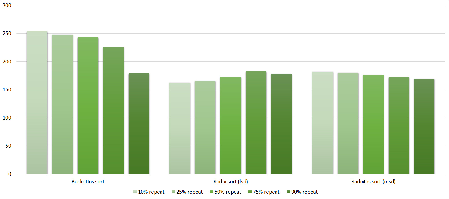
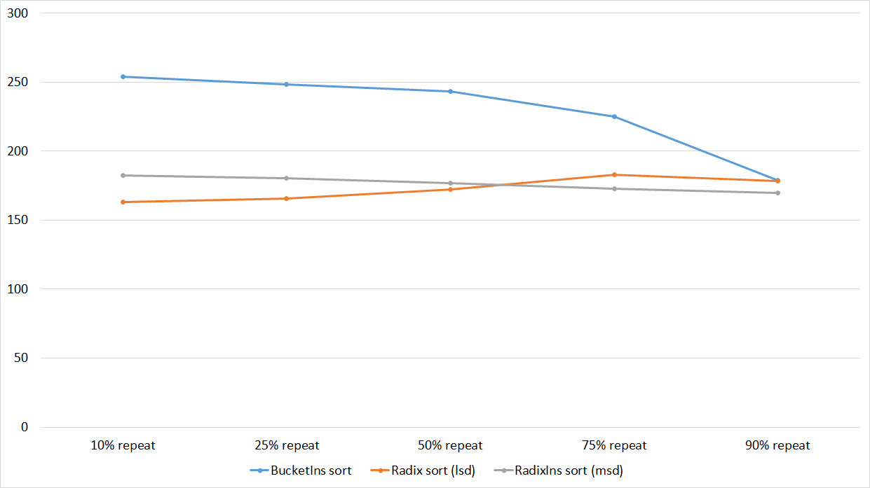

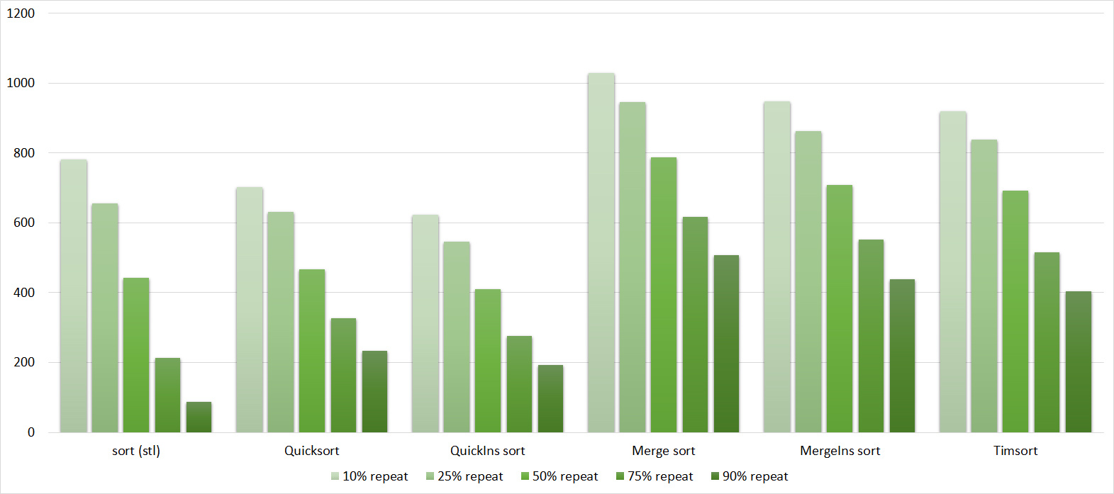


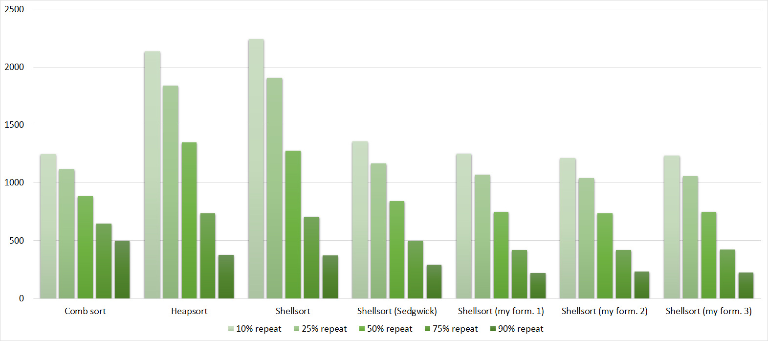
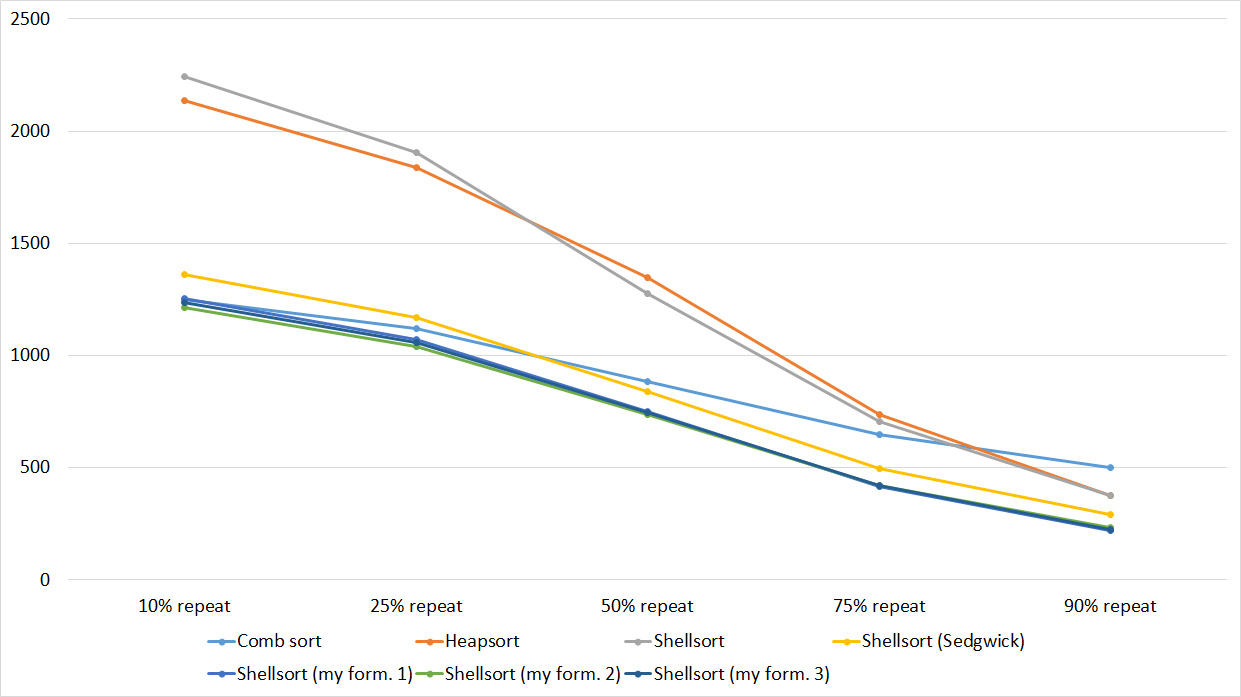
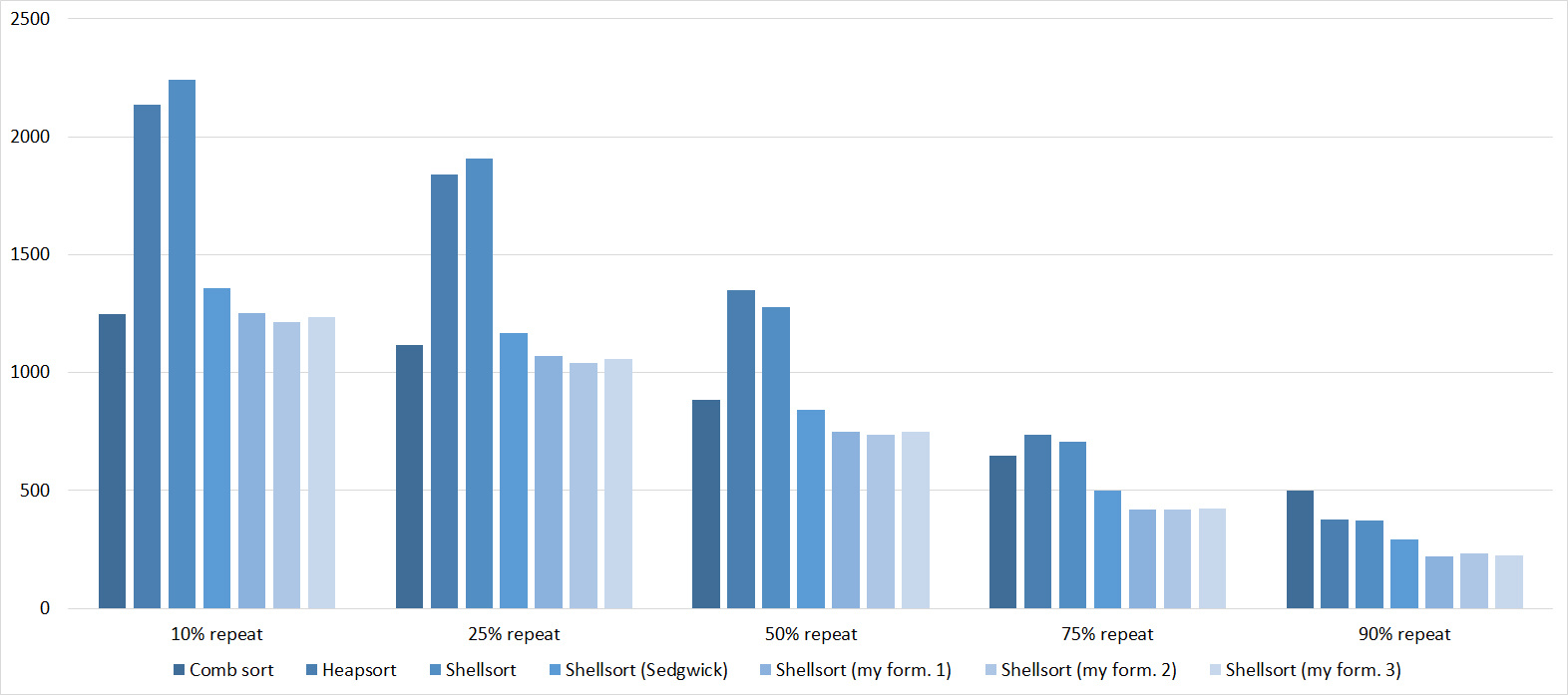
Tables, 1e8 elements


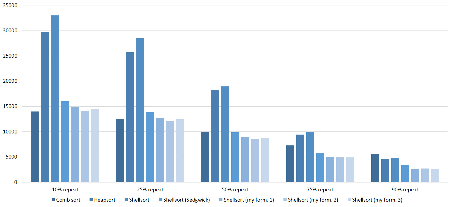
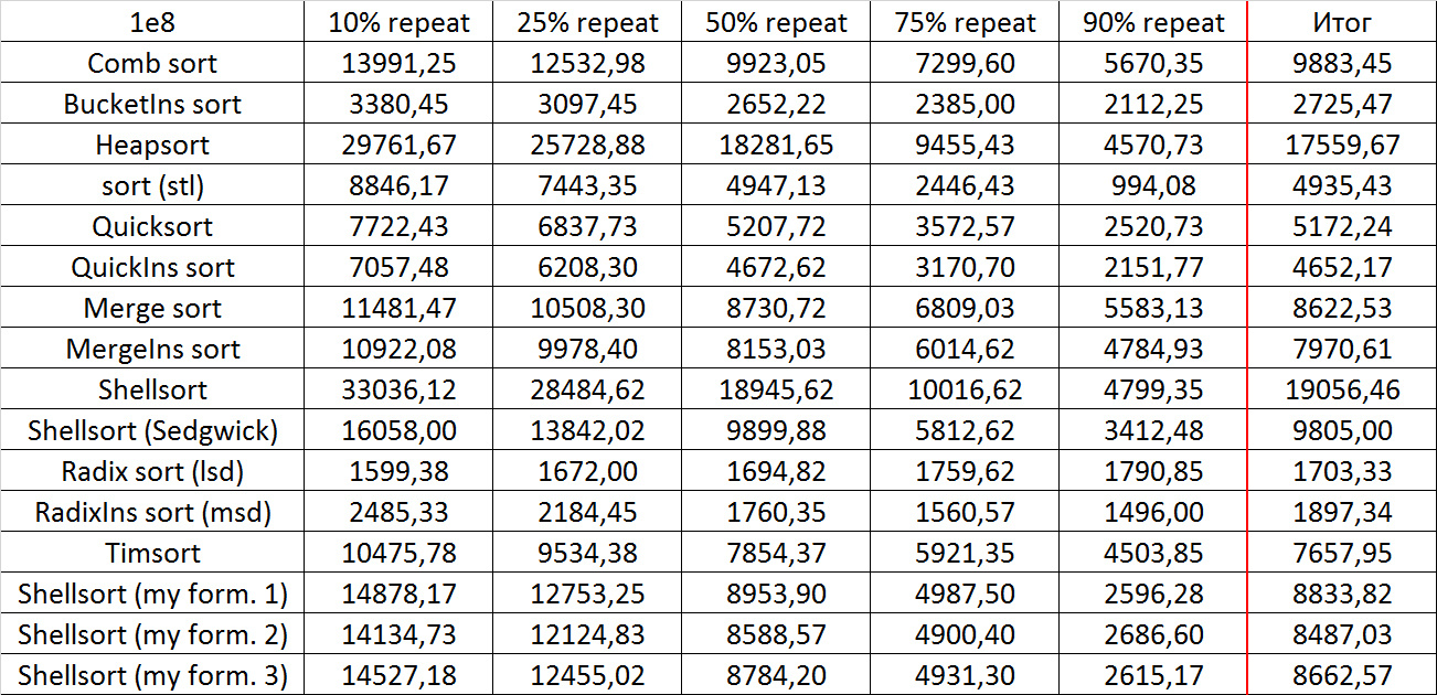
Here everything is rather depressing, all the sortings work with the same dynamics (except linear). From the unusual, it can be seen that the merge sort fell below Shell sort.
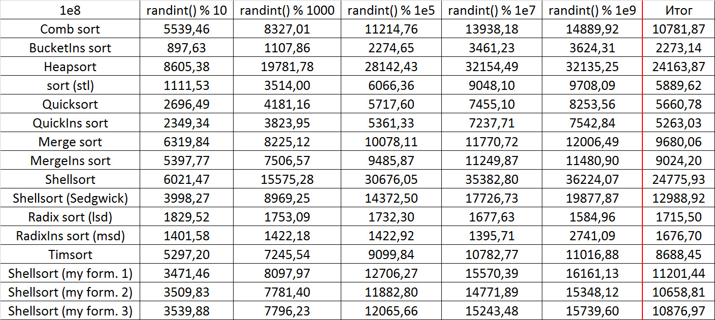
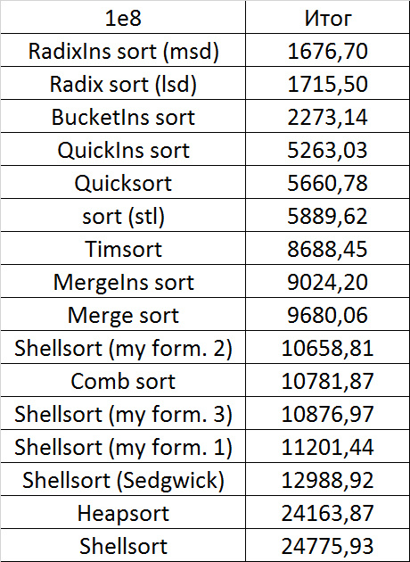
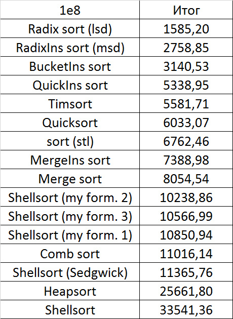
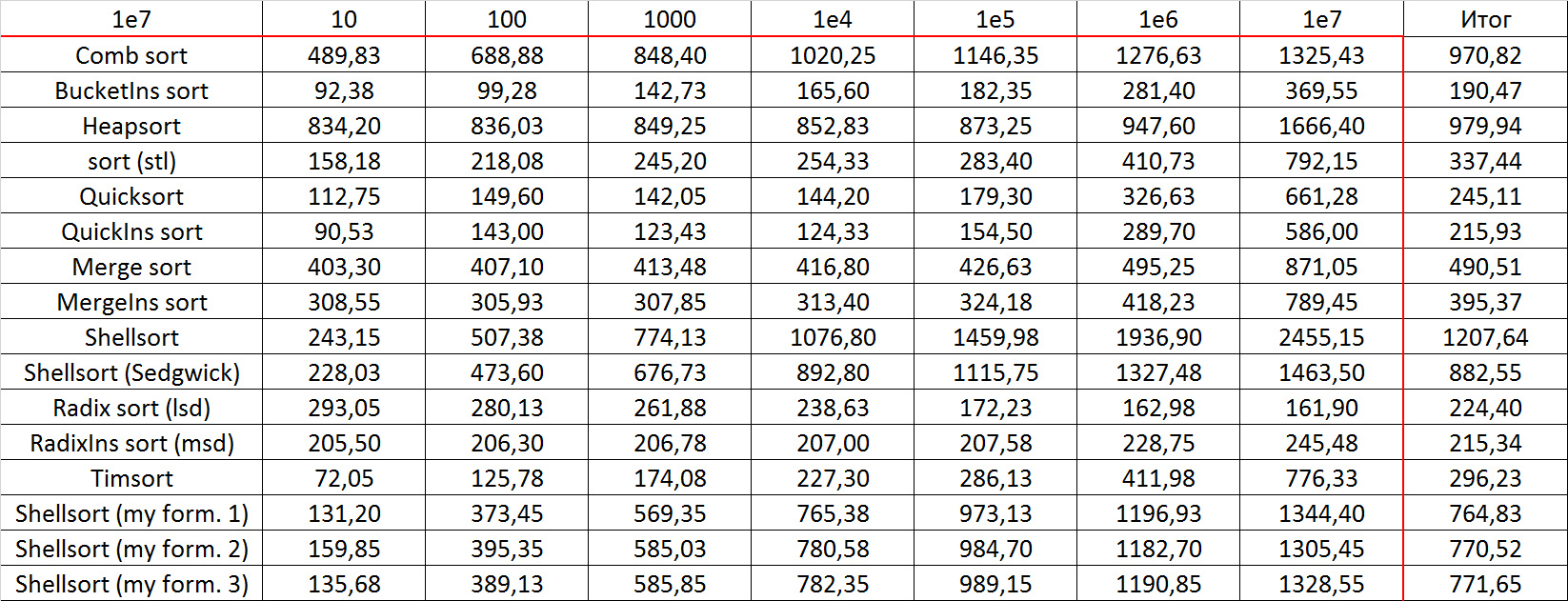
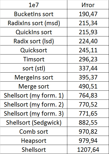
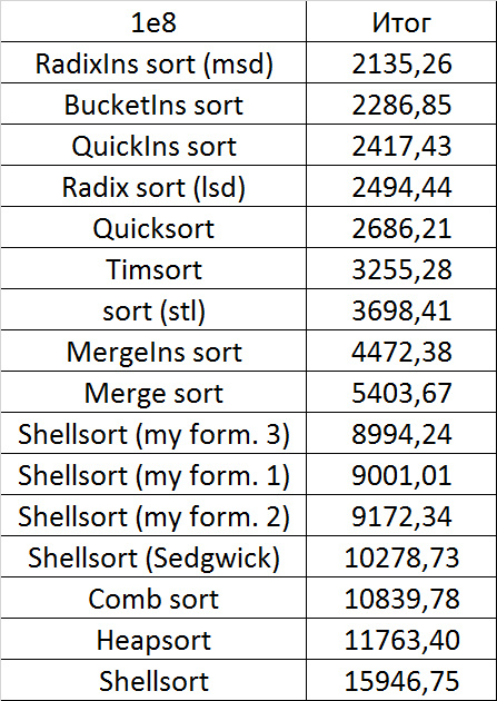
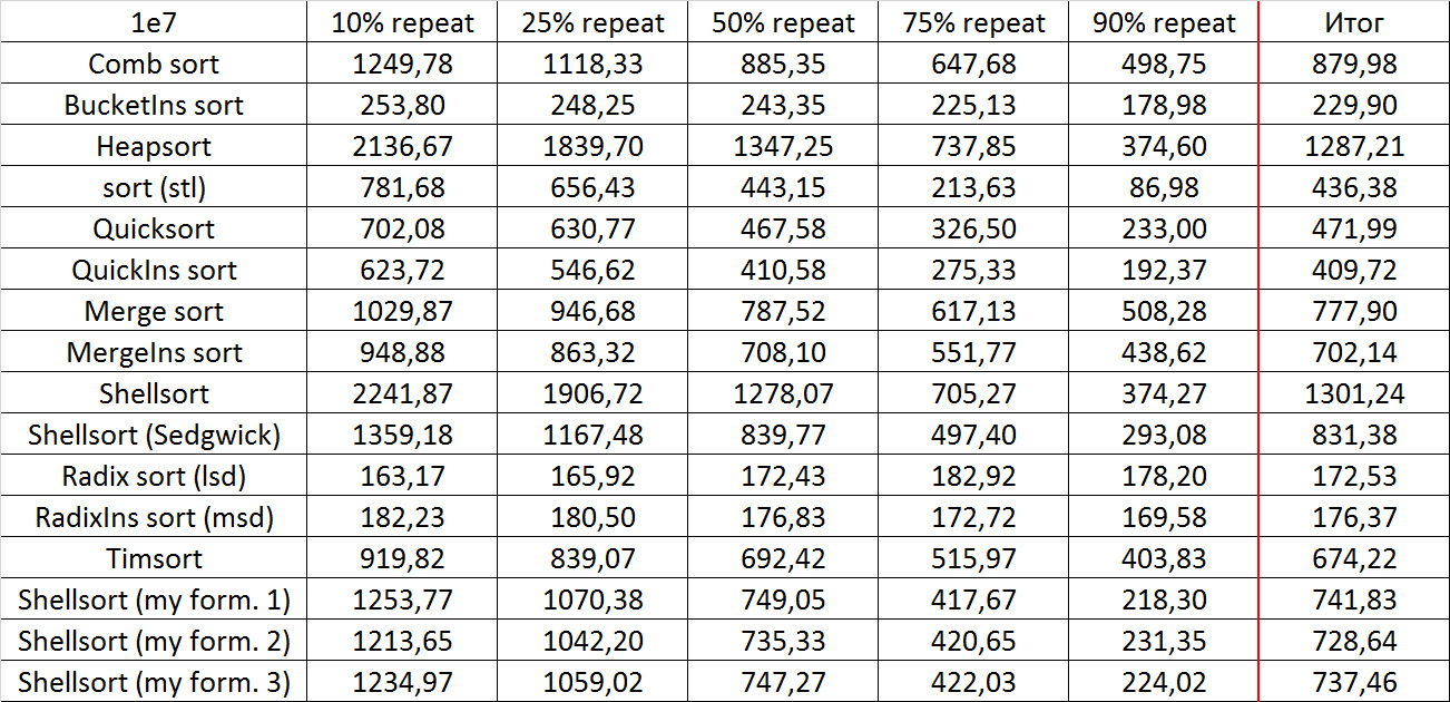
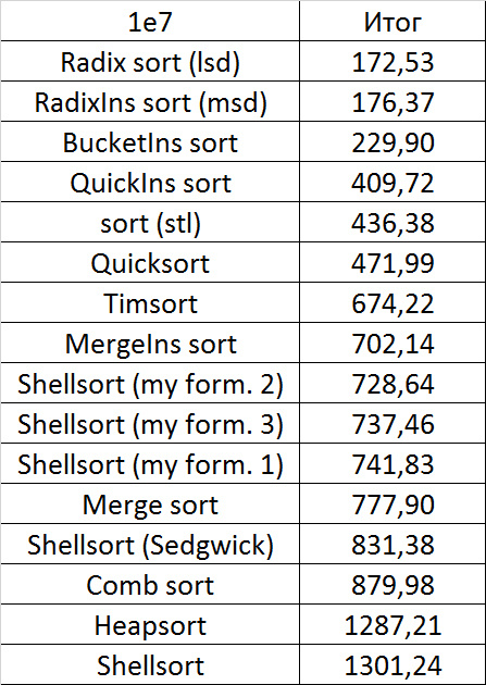
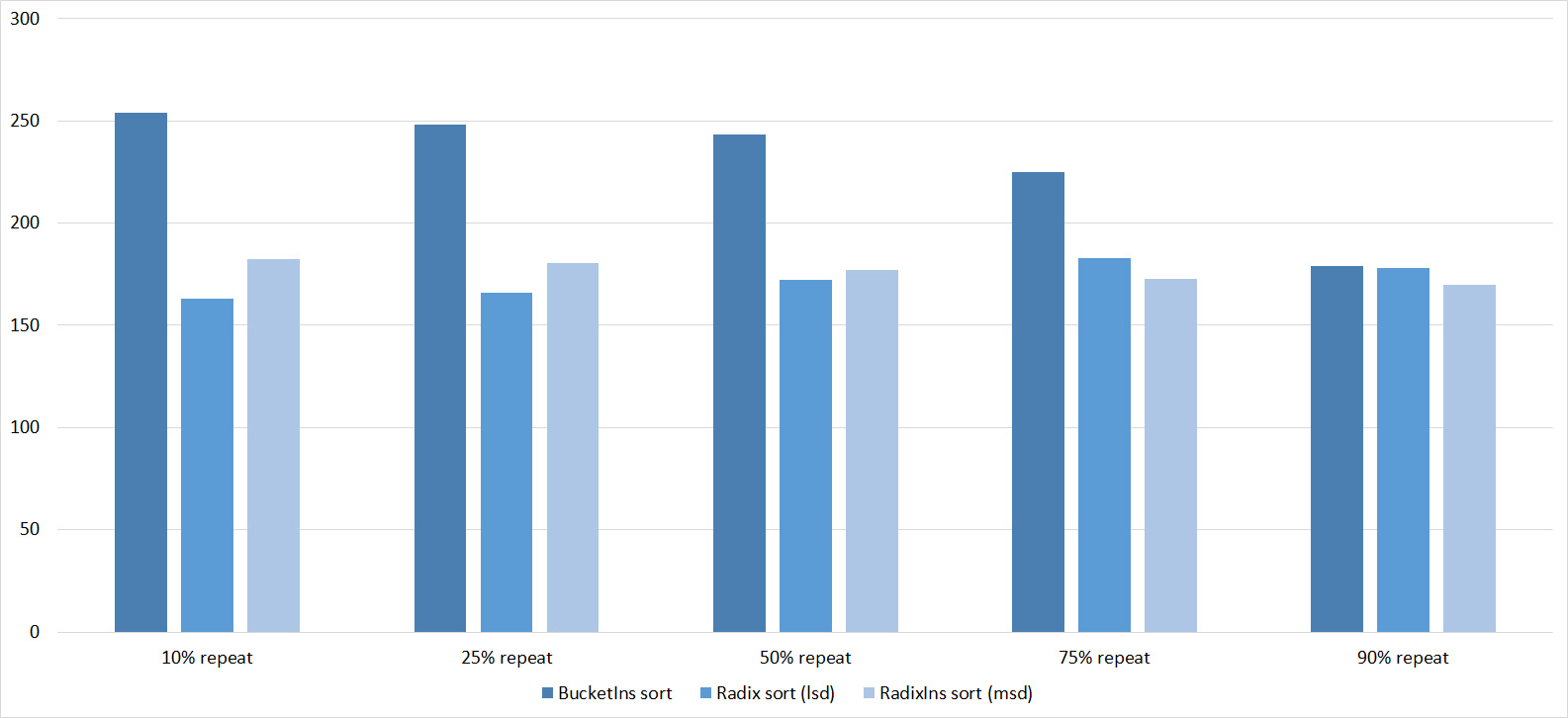
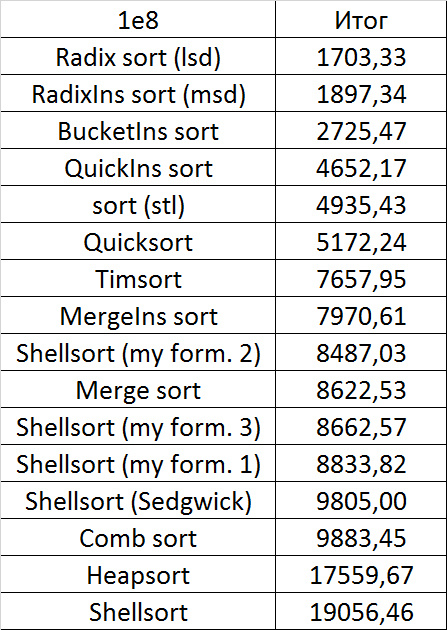
Final results
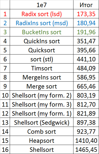

Despite my efforts, the LSD version of the bitwise sorting still took first place at 10 7 and 10 8 elements. She also showed an almost linear increase in time. Her only weakness I noticed is poor work with permutations. The MSD version worked a little worse, primarily due to the large number of tests consisting of random numbers modulo 10 9. I was satisfied with the implementation of block sorting, despite its cumbersome, it showed a good result. By the way, I noticed it too late, it is not fully optimized, you can still separately create run and cnt arrays, so as not to waste time deleting them. Then confidently took the place of various versions of quick sort. Timsort, in my opinion, failed to render them a serious competition, although he was not far behind. Next in speed are merge sorts, after them my versions of Shell sort. The best was the sequence s * 3 + s / 3, where s is the previous element of the sequence. Next comes the only discrepancy in the two tables - the comb sorting turned out to be better with a larger number of elements than Shell sorting with the Sedgwik sequence.And for the last place the pyramid sorting and the original sort of Shell were fighting.
Won the last one. By the way, Shell sorting, as I later checked, works very poorly on tests of size 2 n , so she was just lucky that she was in the first group.
If we talk about practical application, then bitwise sorting (especially the lsd version) is good, it is stable, easy to implement and very fast, but not based on comparisons. Of the sorts based on comparisons, quick sorting looks best. Its drawbacks are instability and quadratic operating time on unsuccessful input data (even if they can occur only with the intentional creation of a test). But this can be dealt with, for example, by choosing a supporting element by some other principle, or by switching to a different sort on failure (for example, introsort, which, if I’m not mistaken, is implemented in C ++). Timsort is devoid of these shortcomings, works better on heavily sorted data, but it’s still slower overall and is much more difficult to write. The remaining sorting at the moment, perhaps, is not very practical. Except, of course,sorting inserts, which can be very well sometimes inserted into the algorithm.
Conclusion
I should note that not all known sortings took part in testing, for example, smooth sorting was missed (I just could not implement it adequately). However, I do not think that this is a big loss, this sorting is very cumbersome and slow, as you can see, for example, from this article: habrahabr.ru/post/133996 You can also explore sorting for parallelization, but, first, I don’t experience, and secondly, the results that were obtained are extremely unstable, the influence of the system is very great.
Here you can see the results of all launches, as well as some auxiliary testing: link to the document .
Here you can see the code of the entire project.
Implementations of algorithms with vectors remained, but I do not guarantee their correctness and good work. It is easier to take the function codes from the article and redo it. Test generators may also not correspond to reality, in fact, they took on this form after the creation of tests, when it was necessary to make the program more compact.
In general, I am pleased with the work done, I hope that you were interested.
Source: https://habr.com/ru/post/335920/
All Articles