Those familiar with public-key cryptography probably know the abbreviations ECC , ECDH and ECDSA . The first is an abbreviation for Elliptic Curve Cryptography (cryptography on elliptic curves), the rest are the names of algorithms based on it.

Today, cryptosystems on elliptic curves are used in TLS , PGP and SSH , the most important technologies on which the modern web and the world of IT are based. I'm not talking about Bitcoin and other cryptocurrencies.
')
Before ECC became popular, almost all public key algorithms were based on RSA, DSA, and DH, alternative cryptosystems based on modular arithmetic. RSA and company are still popular, and are often used with ECC. However, despite the fact that the magic underlying RSA and similar algorithms are easily explained and understandable to many, and coarse implementations are written quite simply , the basics of ECC are still a mystery to most people.

In this series of articles, I will introduce you to the basics of the world of cryptography on elliptic curves. My goal is not to create a complete and detailed guide on ECC (the Internet is full of information on this topic), but a simple review of ECC and an explanation of why it is considered safe . I will not waste time on long mathematical proofs or boring implementation details. I will also provide useful examples with visual interactive tools and scripts .

In particular, I will cover the following topics:

1. Elliptic curves over real numbers and group law
2. Elliptic curves over finite fields and the discrete logarithm problem
3. Generating key pairs and two ECC algorithms: ECDH and ECDSA
4. Algorithms for cracking ECC protection and comparison with RSA

To understand the article, you need to know the basics of set theory, geometry and modular arithmetic, understand the principles of symmetric and asymmetric cryptography. Finally, you must clearly understand what “simple” and “complex” tasks are and their role in cryptography.

Ready? Let's get started!

Part 1: elliptic curves over real numbers and the group law

Elliptic curves

First, what is an elliptic curve? Wolfram MathWorld has an excellent and comprehensive definition . But for us it is enough that the elliptic curve is just a set of points, described by the equation :

$$

$$y ^ 2 = x ^ 3 + ax + b$$

Where $$$4a ^ 3 + 27b ^ 2 \ ne 0$ , (this is necessary to exclude particular curves ). The above equation is called Weierstrass standard formulation for elliptic curves.


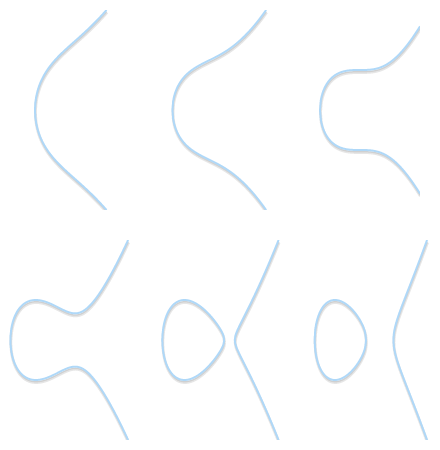
Various forms of elliptic curves ( $$$b = 1$ , $$$a$ varies from 2 to -3).


Types of features: on the left - a curve with a cusp () $$$y ^ 2 = x ^ 3$ ). On the right is a curve with self-intersection ( $$$y ^ 2 = x ^ 3 - 3x + 2$ ). Both of these examples are not full elliptic curves.

Depending on the values $$$a$ and $$$b$ Elliptic curves can take on different shapes on a plane. As you can easily see and check, the elliptic curves are symmetrical about the axis $$$X$ .

For our purposes, we also need the infinite point (also known as the ideal point) to be part of the curve . From now on, we will denote the infinitely remote point by the symbol 0 (zero).

If we need to explicitly consider a point at infinity, then the definition of an elliptic curve can be clarified as follows:

$$

$$\ left \ {(x, y) \ in \ mathbb {R} ^ 2 \ | \ y ^ 2 = x ^ 3 + ax + b, \ 4 a ^ 3 + 27 b ^ 2 \ ne 0 \ right \ } \ \ cup \ \ left \ {0 \ right \}$$

Groups

In mathematics, a group is a set for which we have defined a binary operation, called “addition” and denoted by the symbol +. To set $$$\ mathbb {G}$ was a group, the addition must be defined in such a way that it corresponds to the four following properties:

1. closure: if $$$a$ and $$$b$ enter into $$$\ mathbb {G}$ then $$$a + b$ enters into $$$\ mathbb {G}$ ;
2. associativity: $$$(a + b) + c = a + (b + c)$ ;
3. there exists a unit element 0 such that $$$a + 0 = 0 + a = a$ ;
4. each element has a reciprocal , that is: for each $$$a$ there is such $$$b$ , what $$$a + b = 0$ .

If we add the fifth requirement:

1. commutativity: $$$a + b = b + a$ ,

then the group is called an abelian group .

In the usual record of addition, the set of integers $$$\ mathbb {Z}$ is a group (moreover, it is an abelian group). The set of natural numbers $$$\ mathbb {N}$ However, it is not a group, because it does not satisfy the fourth property.

Groups are convenient because if we prove compliance with all four properties, we will automatically get some other properties "in the load." For example: a single element is unique ; besides, the return values ​​are unique , that is: for each $$$a$ there is only one $$$b$ such that $$$a + b = 0$ (and we can write $$$b$ as $$$-a$ ). Directly or indirectly, these and other properties of groups will be very useful to us in the future.

Group law for elliptic curves

We can define a group for elliptic curves. Namely:

• the elements of a group are points of an elliptic curve;
• the unit element is the infinitely remote point 0;
• return point $$$P$ Is a point symmetrical about the axis $$$x$ ;
• addition is given by the following rule: the sum of three nonzero points $$$P$ , $$$Q$ and $$$R$ lying on one straight line will be equal $$$P + Q + R = 0$ .

The sum of three points on the same line is 0.

It is worth considering that in the last rule we need only three points on one straight line, and the order of arrangement of these three points is not important. This means that if three points $$$P$ , $$$Q$ and $$$R$ lie on one straight line then $$$P + (Q + R) = Q + (P + R) = R + (P + Q) = \ cdots = 0$ . Thus, we intuitively proved that our operator + has the properties of associativity and commutativity: we are in the Abelian group .

So far everything is going great. But how do we calculate the sum of two arbitrary points?

Geometric addition

Due to the fact that we are in an abelian group, we can write $$$P + Q + R = 0$ as $$$P + Q = -R$ . This equation in this form allows us to derive a geometric method for calculating the sum of two points $$$P$ and $$$Q$ : if we draw a line through $$$P$ and $$$Q$ This line will cross the third point of the curve. $$$R$ (this is implied because $$$P$ , $$$Q$ and $$$R$ are on the same line) . If we take the reciprocal of this point $$$-R$ we will find the amount $$$P + Q$ .


We draw straight through $$$P$ and $$$Q$ . The line crosses the third point. $$$R$ . Symmetrical point $$$-R$ is the result $$$P + Q$ .

The geometric method works, but needs improvement. In particular, we need to answer a few questions:

• What if $$$P = 0$ or $$$Q = 0$ ? Of course, we will not be able to draw a straight line (0 is not on the plane $$$xy$ ). But since we defined 0 as a single element, $$$P + 0 = P$ and $$$0 + Q = Q$ for any $$$P$ and any $$$Q$ .
• What if $$$P = -Q$ ? In this case, the straight line passing through two points is vertical and does not intersect the third point. But if $$$P$ is the reciprocal of $$$Q$ then $$$P + Q = P + (-P) = 0$ from the definition of the reciprocal.
• What if $$$P = Q$ ? In this case, an infinite number of straight lines passes through the point. Here, things get a little more complicated. But imagine that point $$$Q '\ ne P$ . What happens if we force $$$Q '$ aspire to $$$P$ getting closer to her?
  
  
  
  
  When two points approach each other, the line passing through them becomes tangent to the curve.
  
  Insofar as $$$Q '$ committed to $$$P$ straight through $$$P$ and $$$Q '$ becomes tangent to the curve. In light of this, we can say that $$$P + P = -R$ where $$$R$ Is the point of intersection between the curve and the tangent to the curve at $$$P$ .
• What if $$$P \ ne Q$ but third point $$$R$ not? In this case, the situation is similar to the previous one. In fact, in this situation the straight line passing through $$$P$ and $$$Q$ , is tangent to a curve.
  
  
  
  
  If our straight line intersects only two points, then this means that it is tangent to the curve. It is easy to see how the result of the addition becomes symmetric to one of two points.
  
  Let's pretend that $$$P$ is a touch point. In the previous case, we recorded $$$P + P = -Q$ . This equation is now turning into $$$P + Q = -P$ . On the other hand, if the touch point were $$$Q$ , then the equation would be correct $$$P + Q = -Q$ .

The geometric method is now complete and takes into account all cases. With the help of a pencil and a ruler, we can perform the addition of all points of any elliptic curve. If you want to try, take a look at the HTML5 / JavaScript visual tool that I created to calculate the sums of elliptic curves .

Algebraic addition

If we want the computer to do the addition of points, we need to turn the geometric method into an algebraic one. Transforming the above rules into a set of equations may seem simple, but in fact it is rather tedious because it requires solving cubic equations. Therefore, I present only the results.

First, let's get rid of the most annoying dead ends. We already know that $$$P + (-P) = 0$ and know that $$$P + 0 = 0 + P = P$ . Therefore, in our equations we will avoid these two cases and consider only two non-zero asymmetric points. $$$P = (x_P, y_P)$ and $$$Q = (x_Q, y_Q)$ .

If a $$$P$ and $$$Q$ do not match ( $$$x_P \ ne x_Q$ ), then the straight line passing through them has a slope :

$$

$$m = \ frac {y_P - y_Q} {x_P - x_Q}$$

The intersection of this line with an elliptic curve is the third point. $$$R = (x_R, y_R)$ :

$$

$$\ begin {array} {rcl} x_R & = & m ^ 2 - x_P - x_Q \\ y_R & = & y_P + m (x_R - x_P) \ end {array}$$

or, similarly:

$$

$$y_R = y_Q + m (x_R - x_Q)$$

therefore $$$(x_P, y_P) + (x_Q, y_Q) = (x_R, -y_R)$ (notice the signs and remember that $$$P + Q = -R$ ).

If we had to check the correctness of the result, we would have to check whether $$$R$ curve and whether $$$P$ , $$$Q$ and $$$R$ on one straight line. Checking the presence on one straight line is trivial, and checking the belonging $$$R$ there is no curve, because we have to solve the cubic equation, which is very sad.

Instead, let's experiment with an example: according to the visual tool , when $$$P = (1, 2)$ and $$$Q = (3, 4)$ belonging curve $$$y ^ 2 = x ^ 3 - 7x + 10$ their sum is equal to $$$P + Q = -R = (-3, 2)$ . Let's check if this corresponds to the equations:

$$

$$\ begin {array} {rcl} m & = & \ frac {y_P - y_Q} {x_P - x_Q} = \ frac {2 - 4} {1 - 3} = 1 \\ x_R & = & m ^ 2 - x_P - x_Q = 1 ^ 2 - 1 - 3 = -3 \\ y_R & = & y_P + m (x_R - x_P) = 2 + 1 \ cdot (-3 - 1) = -2 \\ & = & y_Q + m (x_R - x_Q) = 4 + 1 \ cdot (-3 - 3) = -2 \ end {array}$$

Yes that's right!

Note that these equations work even when the point $$$P$ or $$$Q$ is a touch point . Let's check on $$$P = (-1, 4)$ and $$$Q = (1, 2)$ .

$$

$$\ begin {array} {rcl} m & = & \ frac {y_P - y_Q} {x_P - x_Q} = \ frac {4 - 2} {- 1 - 1} = -1 \\ x_R & = & m ^ 2 - x_P - x_Q = (-1) ^ 2 - (-1) - 1 = 1 \\ y_R & = & y_P + m (x_R - x_P) = 4 + -1 \ cdot (1 - (-1)) = 2 \ end {array}$$

We got the result $$$P + Q = (1, -2)$ that matches the result obtained in the visual tool .

To the occasion $$$P = Q$ need to be treated a little differently : equations for $$$x_R$ and $$$y_R$ remain the same, but given that $$$x_P = x_Q$ we have to use another equation for slope :

$$

$$m = \ frac {3 x_P ^ 2 + a} {2 y_P}$$

Note that, as you might expect, this expression for $$$m$ is the first derivative:

$$

$$y_P = \ pm \ sqrt {x_P ^ 3 + ax_P + b}$$

To prove the correctness of this result, it is enough to make sure that $$$R$ belongs to a curve and that straight line passing through $$$P$ and $$$R$ , has only two intersections with the curve. But again we will not prove it and instead consider an example: $$$P = Q = (1, 2)$ .

$$

$$\ begin {array} {rcl} m & = & \ frac {3x_P ^ 2 + a} {2 y_P} = \ frac {3 \ cdot 1 ^ 2 - 7} {2 \ cdot 2} = -1 \\ x_R & = & m ^ 2 - x_P - x_Q = (-1) ^ 2 - 1 - 1 = -1 \\ y_R & = & y_P + m (x_R - x_P) = 2 + (-1) \ cdot (- 1 - 1) = 4 \ end {array}$$

What gives us $$$P + P = -R = (-1, -4)$ . Right!

Although the procedure for obtaining results is very tedious, our equations are rather short. All this is due to Weierstrass's usual formulation: without it, these equations would be very long and complicated!

Scalar multiplication

In addition to addition, we can define another operation: scalar multiplication , that is:

$$

$$nP = \ underbrace {P + P + \ cdots + P} _ {n \ \ text {times}}$$

Where $$$n$ - natural number. I also wrote a visual tool for scalar multiplication, so you can experiment with it.

When writing in this form, it is obvious that the calculation $$$nP$ requires $$$n$ additions. If a $$$n$ consists of $$$k$ decimal places, the algorithm will have complexity $$$O (2 ^ k)$ that is not very good. But there are faster algorithms.

One of them is the doubling-addition algorithm. The principle of its work is easier to explain with an example. Take $$$n = 151$ . In binary form, it has the form $$$10010111_2$ . Such a binary form can be represented as a sum of powers of two:

$$

$$\ begin {array} {rcl} 151 & = & 1 \ cdot 2 ^ 7 + 0 \ cdot 2 ^ 6 + 0 \ cdot 2 ^ 5 + 1 \ cdot 2 ^ 4 + 0 \ cdot 2 ^ 3 + 1 \ cdot 2 ^ 2 + 1 \ cdot 2 ^ 1 + 1 \ cdot 2 ^ 0 \\ & = & 2 ^ 7 + 2 ^ 4 + 2 ^ 2 + 2 ^ 1 + 2 ^ 0 \ end {array}$$

(We took every binary digit $$$n$ and multiplied by a power of two.)

With this in mind, you can write:

$$

$$151 \ cdot P = 2 ^ 7 P + 2 ^ 4 P + 2 ^ 2 P + 2 ^ 1 P + 2 ^ 0 P$$

The doubling-addition algorithm sets the following procedure:

• To take $$$P$ .
• Double it to get $$$2P$ .
• Lay down $$$2P$ and $$$P$ (to get the result $$$2 ^ 1P + 2 ^ 0P$ ).
• Double up $$$2P$ , To obtain $$$2 ^ 2P$ .
• Add with result (to get $$$2 ^ 2P + 2 ^ 1P + 2 ^ 0P$ ).
• Double up $$$2 ^ 2P$ , receive $$$2 ^ 3P$ .
• Do not add with $$$2 ^ 3P$ .
• Double up $$$2 ^ 3P$ , To obtain $$$2 ^ 4P$ .
• Add with result (to get $$$2 ^ 4P + 2 ^ 2P + 2 ^ 1P + 2 ^ 0P$ ).
• ...

As a result, we calculate $$$151 \ cdot P$ by completing only seven doublings and four additions.

If this is not completely clear to you, then here is a Python script that implements this algorithm:

def bits(n): """    n,     . bits(151) -> 1, 1, 1, 0, 1, 0, 0, 1 """ while n: yield n & 1 n >>= 1 def double_and_add(n, x): """   n * x,   -. """ result = 0 addend = x for bit in bits(n): if bit == 1: result += addend addend *= 2 return result 

If doubling and addition are operations $$$O (1)$ , then this algorithm has complexity $$$O (\ log n)$ (or $$$O (k)$ , considering the bit length), which is pretty good. And, of course, much better than the original algorithm. $$$O (n)$ !

Logarithm

For given $$$n$ and $$$P$ we have at least one polynomial calculation algorithm $$$Q = nP$ . But what about the inverse problem? What if we know $$$Q$ and $$$P$ , and we need to determine $$$n$ ? This task is known as logarithm problem . We use the word “logarithm” instead of the term “division” for consistency with other cryptosystems (in which, instead of multiplication, exponentiation is used).

I do not know of a single “simple” algorithm for solving the logarithm problem, but experimenting with multiplication , it is easy to detect some regularities. For example, take a curve $$$y ^ 2 = x ^ 3 - 3x + 1$ and point $$$P = (0, 1)$ . We can immediately make sure that if $$$n$ odd then $$$nP$ is located on a curve in the left half-plane; if a $$$n$ even, then $$$nP$ - in the right half-plane. If you experiment further, we may find other patterns that lead us to write an algorithm to efficiently calculate the logarithm of this curve.

But there is a variation of the logarithm problem: the discrete logarithm problem. As we will see in the next section, if we reduce the domain of elliptic curves, scalar multiplication remains “simple”, and the discrete logarithm becomes a “difficult” task . This duality is a key feature of cryptography on elliptic curves.

In the next part, we explore finite fields and the problem of discrete logarithmization , as well as examples and tools for experiments.

Part 2: Elliptic curves over finite fields and the discrete logarithm problem

In the previous section, we discussed how elliptic curves over real numbers can be used to define groups. Namely, we determined the rule of addition of points: the sum of three points lying on one straight line is equal to zero ( $$$P + Q + R = 0$ ). We have derived geometric and algebraic methods for calculating the addition of points.

Then we introduced the concept of scalar multiplication ( $$$nP = P + P + \ cdots + P$ ) and found a “simple” algorithm for calculating scalar multiplication: doubling-addition.

Now we will limit the elliptic curves to finite fields , not real numbers, and see what it will change.

Integer field modulo p

The final field is, first of all, the set of a finite number of elements. An example of a finite field is the set of integers modulo $$$p$ where $$$p$ - Prime number. In general, it is written as $$$\ mathbb {Z} / p$ , $$$GF (p)$ or $$$\ mathbb {F} _p$ . We will use the last entry.

For fields there are two double operations: addition (+) and multiplication (·). Both are closed, associative, and commutative. For both operations there is a unique unit element and for each element there is a unique element of the return value. And, finally, multiplication is distributive with respect to addition: $$$x \ cdot (y + z) = x \ cdot y + x \ cdot z$ .

The set of integers modulo $$$p$ consists of all integers from 0 to $$$p - 1$ . Addition and multiplication work as in modular arithmetic . Here are some examples of operations $$$\ mathbb {F} _ {23}$ :

• Addition: $$$(18 + 9) \ bmod {23} = 4$
• Subtraction: $$$(7 - 14) \ bmod {23} = 16$
• Multiplication: $$$4 \ cdot 7 \ bmod {23} = 5$
• Additive inversion: $$$-5 \ bmod {23} = 18$ . Really: $$$(5 + (-5)) \ bmod {23} = (5 + 18) \ bmod {23} = 0$
• Multiplicative inversion: $$$9 ^ {- 1} \ bmod {23} = 18$

If these equations are unfamiliar to you and you want to learn the basics of modular arithmetic, take a course at the Khan Academy .

As we have said the integers modulo $$$p$ - this field, so all the above properties are preserved. Please note that the requirement that $$$p$ It was a prime number, very important! The set of integers modulo 4 is not a field: 2 does not have a multiplicative inversion (i.e., the equation $$$2 \ cdot x \ bmod {4} = 1$ has no solutions).

Modulo p

Soon we will define elliptic curves for $$$\ mathbb {F} _p$ but first we need to clearly understand that $$$x / y$ means over $$$\ mathbb {F} _p$ . Simply put: $$$x / y = x \ cdot y ^ {- 1}$ or, in plain text, $$$x$ in numerator and $$$y$ denominator equals $$$x$ return value $$$y$ . This does not surprise us, but it gives us an easy way to do division: find the reciprocal of a number, and then perform a simple multiplication .

Calculating the inverse number can be "simply" performed using the advanced Euclidean algorithm , which in the worst case is difficult $$$O (\ log p)$ (or $$$O (k)$ if we consider bit length).

We will not go into the details of the advanced Euclidean algorithm, this is not included in the scope of the article, but I will present a working implementation in Python:

 def extended_euclidean_algorithm(a, b): """      (gcd, x, y), ,  a * x + b * y == gcd,  gcd -    a  b.              O(log b). """ s, old_s = 0, 1 t, old_t = 1, 0 r, old_r = b, a while r != 0: quotient = old_r // r old_r, r = r, old_r - quotient * r old_s, s = s, old_s - quotient * s old_t, t = t, old_t - quotient * t return old_r, old_s, old_t def inverse_of(n, p): """    n   p.       m,   (n * m) % p == 1. """ gcd, x, y = extended_euclidean_algorithm(n, p) assert (n * x + p * y) % p == gcd if gcd != 1: #  n  0,  p   . raise ValueError( '{} has no multiplicative inverse ' 'modulo {}'.format(n, p)) else: return x % p 

Elliptic curves over $$$\ mathbb {F} _p$

Now we have all the necessary elements to limit the elliptic curves to the field $$$\ mathbb {F} _p$ . The set of points that in the previous part had the following form:

$$

$$\ begin {array} {rcl} \ left \ {(x, y) \ in \ mathbb {R} ^ 2 \ right. & \ left. | \ right. & \ left. y ^ 2 = x ^ 3 + ax + b, \ right. \\ & & \ left. 4a ^ 3 + 27b ^ 2 \ ne 0 \ right \} \ \ cup \ \ left \ {0 \ right \} \ end {array}$$

now turn into:

$$

$$\ begin {array} {rcl} \ left \ {(x, y) \ in (\ mathbb {F} _p) ^ 2 \ right. & \ left. | \ right. & \ left. y ^ 2 \ equiv x ^ 3 + ax + b \ pmod {p}, \ right. \\ & & \ left. 4a ^ 3 + 27b ^ 2 \ not \ equiv 0 \ pmod {p} \ right \} \ \ cup \ \ left \ {0 \ right \} \ end {array}$$

where 0 is still a point at infinity, and $$$a$ and $$$b$ - two integers in $$$\ mathbb {F} _p$ .


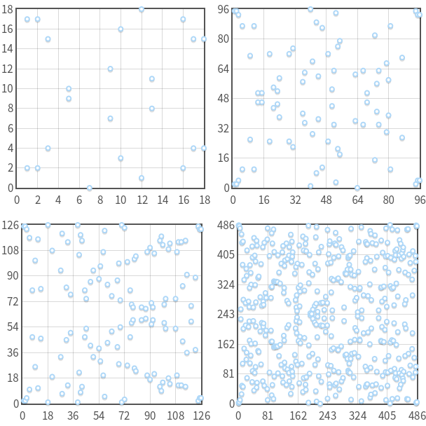
Curve $$$y ^ 2 \ equiv x ^ 3 - 7x + 10 \ pmod {p}$ with $$$p = 19, 97, 127, 487$ . Notice that for each $$$x$ there is a maximum of two points. Also note symmetry regarding $$$y = p / 2$ .


Curve $$$y ^ 2 \ equiv x ^ 3 \ pmod {29}$ - special and has a triple point in $$$(0, 0)$ . It is not a true elliptic curve.

What was previously a continuous curve has now become a multitude of individual points on the plane. $$$xy$ . But it can be proved that despite the limitation of the domain of definition, the elliptic curves over $$$\ mathbb {F} _p$ still create an abelian group .

Addition of points

Obviously, we need to slightly change the definition of addition so that it works for $$$\ mathbb {F} _p$ . For real numbers, we said that the sum of three points on one straight line is zero ( $$$P + Q + R = 0$ ). We can save this definition, but what does it mean that the location of three points on one straight line $$$\ mathbb {F} _p$ ?

We can say that three points are on the same line if there is a line connecting them . Of course, straight over $$$\ mathbb {F} _p$ differ from straight above $$$\ mathbb {R}$ . It can be said that the line is over $$$\ mathbb {F} _p$ - this is a set of points $$$(x, y)$ satisfying the equation $$$ax + by + c \ equiv 0 \ pmod {p}$ (this is the standard equation of a line with an added part " $$$(\ text {mod} \ p)$ ").


Add points for a curve $$$y ^ 2 \ equiv x ^ 3 - x + 3 \ pmod {127}$ at $$$P = (16, 20)$ and $$$Q = (41, 120)$ . Notice how the line connecting the points $$$y \ equiv 4x + 83 \ pmod {127}$ "Repeats" itself on the plane.

Considering the fact that we are still in the group, the addition of points preserves the properties already known to us:

• $$$Q + 0 = 0 + Q = Q$ (from the definition of a single element).
• For $$$Q$ return value $$$-Q$ - This is a point that has the same abscissa, but the opposite ordinate. Or, if you like, $$$-Q = (x_Q, -y_Q \ bmod {p})$ . For example, if the curve is over $$$\ mathbb {F} _ {29}$ has a point $$$Q = (2, 5)$ , then the reciprocal will be $$$-Q = (2, -5 \ bmod {29}) = (2, 24)$ .
• Besides, $$$P + (-P) = 0$ (from the definition of the reciprocal).

Algebraic sum

The equations for performing additions of points are exactly the same as in the previous part , except that we need to add at the end of each expression " $$$\ text {mod} \ p$ ". Therefore, if $$$P = (x_P, y_P)$ , $$$Q = (x_Q, y_Q)$ and $$$R = (x_R, y_R)$ then $$$P + Q = -R$ can be calculated as follows:

$$

$$\ begin {array} {rcl} x_R & = & (m ^ 2 - x_P - x_Q) \ bmod {p} \\ y_R & = & [y_P + m (x_R - x_P)] \ bmod {p} \\ & = & [y_Q + m (x_R - x_Q)] \ bmod {p} \ end {array}$$

If a $$$P \ ne Q$ then slope $$$m$ takes the form:

$$

$$m = (y_P - y_Q) (x_P - x_Q) ^ {- 1} \ bmod {p}$$

Otherwise, if $$$P = Q$ , we get:

$$

$$m = (3 x_P ^ 2 + a) (2 y_P) ^ {- 1} \ bmod {p}$$

The equations have not changed, and this is not a coincidence: in fact, these equations work on any field, both on finite and infinite (except $$$\ mathbb {F} _2$ and $$$\ mathbb {F} _3$ which are special cases). I feel that this needs to be explained. But there is a problem: complex mathematical concepts are usually required to prove a group law. However, I found the proof of Stefan Friedl in which only the simplest concepts are used. Read it if you are wondering why these equations work (almost) on any field.

Let us return to the curves - we will not define the geometric method: in fact, problems will arise with it. For example, in the previous section, we said that to calculate $$$P + P$ we have to take the tangent to the curve in $$$P$ . But in the absence of continuity, the word “tangent” loses all meaning. We may find a way around this and other problems, but a purely geometric method will be too complicated and completely impractical.

Instead, you can experiment with an interactive tool written by me to perform addition of points .

The order of the elliptic curve group

We said that an elliptic curve defined over a finite field has a finite number of points. We need to answer the important question: how many points are there in it?

First, let's determine that the number of points in a group is called the order of the group .

Check all possible values ​​for $$$x$ in the range from 0 to $$$p - 1$ would be an impossible way to count the points, because it would require $$$O (p)$ steps, and this task is “difficult” if $$$p$ - large prime number.

Fortunately, there is a faster algorithm to calculate the order: the Shuf algorithm . I will not go into its details - the main thing is that it is executed in polynomial time, and this is precisely what we need.

Scalar multiplication and cyclic subgroups

For real numbers, multiplication can be defined as:

$$

$$n P = \ underbrace {P + P + \ cdots + P} _ {n \ \ text {times}}$$

And, again, we can use the doubling-addition algorithm to perform multiplication in $$$O (k)$ where $$$k$ Is the number of bits $$$n$ ). I wrote an interactive tool for scalar multiplication .

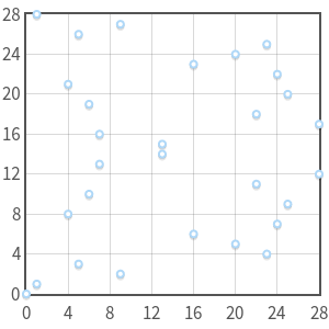
Multiplication of points for elliptic curves over $$$\ mathbb {F} _p$ has an interesting property. Take a curve $$$y ^ 2 \ equiv x ^ 3 + 2x + 3 \ pmod {97}$ and point $$$P = (3, 6)$ . Now let's calculate all multiples. $$$P$ :


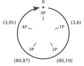
All multiples $$$P = (3, 6)$ , represent five different points ( $$$0$ , $$$P$ , $$$2P$ , $$$3P$ , $$$4P$ ), which are cyclically repeated. It is easy to notice the similarity between scalar multiplication for elliptic curves and addition in modular arithmetic.

• $$$0P = 0$
• $$$1P = (3, 6)$
• $$$2P = (80, 10)$
• $$$3P = (80, 87)$
• $$$4P = (3, 91)$
• $$$5P = 0$
• $$$6P = (3, 6)$
• $$$7P = (80, 10)$
• $$$8P = (80, 87)$
• $$$9P = (3, 91)$
• ...

You can immediately notice two features: first, multiples $$$P$ , only five: the other points of the elliptic curve never become them. Secondly, they are repeated cyclically . You can write:

• $$$5kP = 0$
• $$$(5k + 1) P = P$
• $$$(5k + 2) P = 2P$
• $$$(5k + 3) P = 3P$
• $$$(5k + 4) P = 4P$

for any whole $$$k$ . Note that, thanks to the division operator with the remainder, these five equations can be “pressed” into one: $$$kP = (k \ bmod {5}) P$ .

Moreover, we can immediately show that these five points are closed with respect to the addition operation . What does it mean: no matter how I summed up $$$0$ , $$$P$ , $$$2P$ , $$$3P$ or $$$4P$ The result will always be one of these five points. Again, all other points of an elliptic curve never become a result.

The same applies to all other points, not only $$$P = (3, 6)$ . Actually, if we take $$$P$ in general:

$$

$$nP + mP = \ underbrace {P + \ cdots + P} _ {n \ \ text {times}} + \ underbrace {P + \ cdots + P} _ {m \ \ text {times}} = (n + m) P$$

Which means: if we add two multiples $$$P$ then we get the value multiple $$$P$ (i.e. multiples $$$P$ , closed with respect to the operation of addition). This is enough to prove that the set of multiples $$$P$ Values ​​is a cyclic subgroup of a group formed by an elliptic curve.

A “subgroup” is a group that is a subset of another group. “Cyclic subgroup” is a subgroup whose elements are cyclically repeated, as we showed in the previous example. Point $$$P$ is called a generator or base point of a cyclic subgroup.

Cyclic subgroups are the foundation for ECC and other cryptosystems. Later I will explain why this is so.

Subgroup order

One may ask, what is the order of the subgroup generated by a point $$$P$ (or, in other words, what is the order $$$P$ ). We cannot use the Shuf algorithm to answer this question, because this algorithm works only for entire elliptic curves, but not for subgroups. Before we begin to solve the problem, we need some more information:

• So far we have defined the order as the number of points of the group. This definition is still valid, but in cyclic subgroups we can give a new analogous definition: order $$$P$ Is the minimum positive integer $$$n$ such that $$$nP = 0$ .
  
  In fact, if you look at the previous example, our subgroup consisted of five points, and $$$5P = 0$ .
• Order $$$P$ is connected with the order of the elliptic curve by the Lagrange theorem , according to which the order of the subgroup is a divisor of the order of the original group .
  
  In other words, if the elliptic curve contains $$$N$ points, and one of the subgroups contains $$$n$ then $$$n$ is a divider $$$N$ .

These two facts together enable us to determine the order of the subgroup with the base point. $$$P$ :

1. Calculate the order of an elliptic curve $$$N$ using the Shuf algorithm.
2. Find all dividers $$$N$ .
3. For each divider $$$n$ order $$$N$ we calculate $$$nP$ .
4. Least $$$n$ such that $$$nP = 0$ , is the order of the subgroup.

For example, the curve $$$y ^ 2 = x ^ 3 - x + 3$ over the field $$$\ mathbb {F} _ {37}$ has order $$$N = 42$ . Its subgroups may have order $$$n = 1$ , $$$2$ , $$$3$ , $$$6$ , $$$7$ , $$$14$ , $$$21$ or $$$42$ . If we substitute $$$P = (2, 3)$ then we will see that $$$P \ ne 0$ , $$$2P \ ne 0$ , ..., $$$7P = 0$ i.e. order $$$P$ equals $$$n = 7$ .

Note that it is important to take the smallest, not the random, divider . If we choose randomly, we can get $$$n = 14$ that is not a subgroup order, but is one of multiples.

Another example: an elliptic curve defined by an equation $$$y ^ 2 = x ^ 3 - x + 1$ over the field $$$\ mathbb {F} _ {29}$ has order $$$N = $ 3$ which is a prime number. Its subgroups can only have order $$$n = 1$ or $$$37$ . As you can guess when $$$n = 1$ The subgroup contains only an infinitely distant point; when $$$n = n$ The subgroup contains all points of an elliptic curve.

Base point search

ECC algorithms require high order subgroups. Therefore, an elliptic curve is usually chosen, its order is calculated ( $$$N$ ), as a group order ( $$$n$ ) a large divider is selected, and then a suitable base point is found. That is, we do not choose a base point, after which we calculate its order, but perform the inverse operation: first we choose a reasonably good order, and then we look for a suitable base point. How to do it?

First, you need to introduce another concept. The Lagrange theorem implies that the number $$$h = n / n$ always whole (because $$$n$ - divider $$$N$ ). Number $$$h$ has its own name: it is a cofactor of the subgroup

Now consider that for each point of the elliptic curve there is $$$NP = 0$ . This is true because $$$N$ Is a multiple of any possible $$$n$ . Based on the definition of a cofactor, we can write:

$$

$$n (hP) = 0$$

Now let's say that $$$n$ - a prime number (we prefer simple orders for the reasons stated in the first part of the article). This equation, written in this form, tells us that the dot $$$G = hP$ creates a subgroup of order $$$n$ (except in the case of $$$G = hP = 0$ in which the subgroup has order 1).

In light of this, we can determine the following algorithm:

1. We calculate the order $$$N$ elliptic curve.
2. Choose order $$$n$ subgroups. For the algorithm to work, the number must be simple and be a divisor. $$$N$ .
3. Calculate the cofactor $$$h = n / n$ .
4. Choose a random point on the curve $$$P$ .
5. Calculate $$$G = hP$ .
6. If a $$$G$ equal to 0, then we return to step 4. Otherwise, we have found the generator of the subgroup with the order $$$n$ and cofactor $$$h$ .

Note that the algorithm only works if $$$n$ simple. If $$$n$ wasn't simple then order $$$G$ could be one of the dividers $$$n$ .

Discrete logarithm

As in the case of continuous elliptic curves, we now have to discuss the following question: if we know $$$P$ and $$$Q$ what will be $$$k$ such that $$$Q = kP$ ?

This task, known as the discrete logarithm problem for elliptic curves, is considered “complex”, for which no polynomial time algorithm running on a classical computer has been detected. However, this point of view has no mathematical evidence.

This task is similar to the discrete logarithm problem used in other cryptosystems, such as Digital Signature Algorithm (DSA), Diffie-Hellman Protocol (DH), and El-Gamal scheme. The names of the tasks do not coincide. Their difference is that these algorithms do not use scalar multiplication, but exponentiation modulo. Their discrete logarithm problem can be formulated as follows: if known $$$a$ and $$$b$ what will be $$$k$ such that $$$b = a ^ k \ bmod {p}$ ?

Both of these tasks are “discrete” because they use finite sets (and more specifically, cyclic subgroups). And they are “logarithms” because they are similar to regular logarithms.

ECC is interesting because at the moment the task of discrete logarithm for elliptic curves seems to be “more difficult” compared to other similar tasks used in cryptography. This implies that we need less bits for the whole. $$$k$ to get the same level of protection as in other cryptosystems, and we will look at it in detail in the fourth, last, part of the article.

Part 3: ECDH and ECDSA

Scope parameters

Algorithms of elliptic curves will work in a cyclic subgroup of an elliptic curve over a finite field. Therefore, the algorithms will require the following parameters:

• Simple $$$p$ specifying the size of the final field.
• Coefficients $$$a$ and $$$b$ equations of an elliptic curve.
• $$$G$ generating subgroup.
• Order $$$n$ subgroups.
• Cofactor $$$h$ subgroups.

As a result, the parameters of the domain for the algorithms are six $$$(p, a, b, G, n, h)$ .

Random curves

When I said that the discrete logarithm problem is “complex,” I was not entirely accurate. There are certain classes of elliptic curves that are rather weak and allow using special algorithms to effectively solve the problem of discrete logarithmization. For example, all curves for which$$p = h n (i.e. the order of the final field is equal to the order of the elliptic curve), vulnerable toSmart's attack, which can be used to solve discrete logarithms in polynomial time on classical computers.Suppose now that I gave you the parameters of the curve definition domain. There is a possibility that I discovered a new class of weak curves unknown to no one, and perhaps I created a “fast” algorithm for calculating discrete logarithms for my curve. How can I convince you of the opposite, i.e. is that I don't know about vulnerabilities?How can I guarantee that the curve is “protected” (in the sense that I cannot use it for my own attacks)?$p = hn$



To solve this problem, sometimes you have to use the additional parameter of the definition domain: the seed value $$$S$ . This is a random number used to generate coefficients. $$$a$ and $$$b$ or base point$$$G$ , or both. These parameters are generated by hash calculation.$$$S$ . Heshes, as we know, are “easy” to calculate, but “difficult” to reverse.


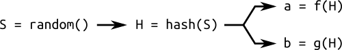
A simple scheme for generating a random curve from a generator value: a hash of a random number is used to calculate various parameters of the curve.


If we wanted to cheat and recreate the hash from the parameters of the domain of definition, then we would have to solve the “complex” problem: inverse of the hash.

The curve generated by the generator value is called testable random . The principle of using hashes to generate parameters is known as " nothing up my sleeve " ("there is nothing in the sleeves"), and is widely used in cryptography.

This trick gives a certain guarantee that the curve was not specially created in such a way as to have vulnerabilities known to its author . In fact, if I give you a curve along with a generating value, it means that I could not arbitrarily choose the parameters$$$a$ and $$b , and you can be relatively calm that I can not use special attacks. The reason for using the word “relatively” will be explained in the fourth part. A standardized algorithm for generating and testing random curves is described in ANSI X9.62 and is based onSHA-1. If interested, you can read about the generation of checkable random curves inthe SECG specification(see “Verifiably Random Curves and Base Point Generators”). I wrote a small Python script that checks all the random curves that are currently shipped with OpenSSL . I highly recommend to watch it!$b$

Cryptography on elliptic curves

We spent a lot of time, but finally got there! It's simple:

1. The private key is a random integer.$$$d$ selected from$$$\{1, \dots, n - 1\}$ (Where $$$n$ is the order of the subgroup).
2. The public key is the point$$$H = dG$ (Where $$$G$ is the base point of the subgroup).

Do you see? If we know $$$d$ and $$$G$ (along with other parameters of the definition domain), then find$$$H$ "just." But if we know$$$H$ and $$$G$ , thensearch for the private key $$$d$ is a “difficult” task because it requires solving a discrete logarithm problem.

Now we describe two public key algorithms based on this principle: ECDH (Elliptic curve Diffie-Hellman, Diffie-Hellman protocol on elliptic curves) used for encryption, and ECDSA (Elliptic Curve Digital Signature Algorithm) used for digital signatures.

ECDH Encryption

ECDH is a variation of the Diffie-Hellman algorithm for elliptic curves. In fact, it is rather a key agreement protocol , rather than an encryption algorithm. In essence, this means that ECDH defines (to a certain extent) the order in which keys are generated and exchanged. We can choose the way to encrypt data using such keys.

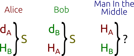
He solves the following problem: the two parties (usually Alice and Bob ) want to safely exchange information so that a third party ( intermediary, Man In the Middle ) can intercept it, but cannot decipher it. For example, this is one of the principles of TLS.

Here's how it works:

1. First, Alice and Bob generate their own private and public keys . Alice has a private key$$$d_A$ $$$H_A = d_AG$ , $$$d_B$ and $$$H_B = d_BG$ . , , : $$$G$ .
2. $$$H_A$ and $$$H_B$ . (Man In the Middle) $$$H_A$ and $$$H_B$ , $$$d_A$ , $$$d_B$ , .
3. $$$S = d_A H_B$ (using Bob’s own private key and Bob’s public key),and Bob calculates $$$S = d_B H_A$ (using Alice’s own private key and Alice’s public key). Please note that$$S is the same for both Alice and Bob. In fact:$S$
   
   

   $$

   $$S = d_A H_B = d_A (d_B G) = d_B (d_A G) = d_B H_A$$

However, the mediator is known only $$$H_A$ and $$H B (along with other parameters of the definition domain) and he will not be able to find theshared secret key$H_B$ $$$S$ . This is known as the Diffie-Hellman problem, which can be stated as follows:

What will be the result $$a b P for three points$abP$$$$P$ , $$$aP$ and $$$bP$ ?

Or similarly:

What will be the result $$k x y for three integers$k^{xy}$$$$k$ , $$$k^x$ and $$$k^y$ ?

(The latter formulation is used in the original Diffie-Hellman algorithm based on modular arithmetic.)


Diffie-Hellman protocol: Alice and Bob can “just” calculate the common secret key, while the mediator will have to solve the “complex” problem.

The principle underlying the Diffie-Hellman problem is also explained in the excellent video of the Hahn Academy on YouTube , which later explains the Diffie-Hellman algorithm applied to modular arithmetic (not to elliptic curves).

The Diffie-Hellman problem for elliptic curves is considered “complex”. It is believed that it is just as “complex” as the discrete logarithm problem, but there is no mathematical proof of this. We can only say with confidence that it cannot be “more difficult”, because solving the logarithm problem is a way to solve the Diffie-Hellman problem.

After receiving a shared secret key, Alice and Bob can exchange data with symmetric encryption.

For example, they can use the coordinate$$x key$x$$$S as a key for encrypting messages with secure cipher keys such asAESor3DES. This is what TLS does, the difference is that TLS connects the coordinate$S$$$x with other numbers related to the connection, and then calculates the hash of the resulting byte string.$x$

Experiments with ECDH

I wrote another Python script to compute private / public keys and shared secret keys over an elliptic curve .

Unlike the examples shown earlier, this script uses a standardized curve, not a simple curve on a small field. I chose the curve secp256k1group SECG ( «Standards for Efficient Cryptography Group is», based Certicom ). The same curve is used in Bitcoin for digital signatures. Here are the scope parameters:

• $$p = 0xffffffff ffffffff ffffffff ffffffff ffffffff ffffffff fffffffe fffffc2f$p$
• $$a = 0$a$
• $$b = 7$b$
• $$x G = 0x79be667e f9dcbbac 55a06295 ce870b07 029bfcdb 2dce28d9 59f2815b 16f81798$x_G$
• $$y G = 0x483ada77 26a3c465 5da4fbfc 0e1108a8 fd17b448 a6855419 9c47d08f fb10d4b8$y_G$
• $$n = 0xffffffff ffffffff ffffffff fffffffe baaedce6 af48a03b bfd25e8c d0364141$n$
• $$$h$ = 1

(These numbers are taken from the OpenSSL source code .)

Of course, you can change the script and use other curves and definition domain parameters, just be sure to use simple fields and Weierstrass wording, otherwise the script will not work.

The script is very simple and contains some of the algorithms described above: point addition, doubling-addition, ECDH. I recommend to study and run it. It creates something like this:

 Curve: secp256k1 Alice's private key: 0xe32868331fa8ef0138de0de85478346aec5e3912b6029ae71691c384237a3eeb Alice's public key: (0x86b1aa5120f079594348c67647679e7ac4c365b2c01330db782b0ba611c1d677, 0x5f4376a23eed633657a90f385ba21068ed7e29859a7fab09e953cc5b3e89beba) Bob's private key: 0xcef147652aa90162e1fff9cf07f2605ea05529ca215a04350a98ecc24aa34342 Bob's public key: (0x4034127647bb7fdab7f1526c7d10be8b28174e2bba35b06ffd8a26fc2c20134a, 0x9e773199edc1ea792b150270ea3317689286c9fe239dd5b9c5cfd9e81b4b632) Shared secret: (0x3e2ffbc3aa8a2836c1689e55cd169ba638b58a3a18803fcf7de153525b28c3cd, 0x43ca148c92af58ebdb525542488a4fe6397809200fe8c61b41a105449507083) 

Ephemeral ECDH

Some of you may have heard of ECDHE, not ECDH. “E” in ECHDE stands for “Ephemeral” (ephemeral) and is due to the fact that the transmitted keys are temporary and not static.

ECDHE is used, for example, in TLS, where the client and server generate their private-public key pair on the fly, when a connection is established. The keys are then signed with a TLS certificate (for authorization) and transferred between the parties.

Signing up with ECDSA

The script is as follows: Alice wants to sign the message with her private key ($$d A ), andBob wants to verify the signature using Alice’s public key($d_A$$$$H_A$ ).No one but Alice should be able to create valid signatures. Everyone should be able to verify signatures.

Alice and Bob reuse the same definition domain parameters. We consider the ECDSA algorithm, a kind of Digital Signature Algorithm applied to elliptic curves.

ECDSA works with the message hash, not with the message itself. The choice of the hash function remains with us, but, obviously, you need to choose a cryptographic hash function . The message hash must be trimmed so that the bit length of the hash is the same as the bit length$$n (subgroup order). The truncated hash is an integer and will be denoted as$n$ $$$z$ .

Alice's algorithm for signing a message works as follows:

1. Take a random integer $$$k$ selected from$$$\{1, \dots, n - 1\}$ (Where $$n is still the order of the group).$n$
2. Calculate point $$$P = kG$ (Where $$G is the base point of the subgroup).$G$
3. Calculate the number $$$r = x_P \bmod{n}$ (Where $$x P is the coordinate$x_P$$$$x$$$$P$ ).
4. If a $$r = 0 , then choose another$r = 0$$$k and try again.$k$
5. Calculate $$$s = k^{-1} (z + rd_A) \bmod{n}$ (Where $$d A is Alice's private key, and$d_A$$$k - 1 - multiplicative inversion$k^{-1}$$$k modulo$k$$$$n$ ).
6. If a $$s = 0 , then choose another$s = 0$$$k and try again.$k$

Couple $$$(r, s)$ is a signature.


Alice signs a hash $$$z$ with the private key $$$d_A$ and random $$$k$ . Bob verifies that the message is signed using Alice’s public key. $$$H_A$ .

Simply put, this algorithm first generates a secret key ( $$$k$ ). Thanks to the multiplication of points (which, as we know, is “simple” in one direction and “difficult” in the opposite direction), the secret key is hidden in $$$r$ . Then $$r is attached to the message hash by the equation$r$$$$s = k^{-1} (z + rd_A) \bmod{n}$ .

Note that to calculate $$s we calculated the reciprocal$s$$$k modulo$k$$$$n$ . As mentioned in the previous part, this is guaranteed to work only if $$n is a prime number. If the subgroup has a non-prime number order, ECDSA cannot be used. It is no coincidence that all standardized curves have a simple order, and those having a complicated order are not applicable to ECDSA.$n$

Signature verification

Alice's public key is required to verify the signature. $$H A , (trimmed) hash$H_A$$$z and obviously the signature$z$$$$(r, s)$ .

1. Calculate the whole $$$u_1 = s^{-1} z \bmod{n}$ .
2. Calculate the whole $$$u_2 = s^{-1} r \bmod{n}$ .
3. Calculate point $$$P = u_1 G + u_2 H_A$ .

Signature is valid only $$$r = x_P \bmod{n}$ .

Algorithm correctness

At first glance, the logic of the algorithm may not be obvious, but if we combine all the equations we have previously written, everything becomes clearer.

Let's start with$$$P = u_1 G + u_2 H_A$ . From the definition of a public key, we know that $$$H_A = d_A G$ (Where $$d A - private key). You can write:$d_A$

$$

$$\begin{array}{rl} P & = u_1 G + u_2 H_A \\ & = u_1 G + u_2 d_A G \\ & = (u_1 + u_2 d_A) G \end{array}$$

In view of the definitions $$$u_1$ and $$u 2 can be written:$u_2$

$$

$$\begin{array}{rl} P & = (u_1 + u_2 d_A) G \\ & = (s^{-1} z + s^{-1} r d_A) G \\ & = s^{-1} (z + r d_A) G \end{array}$$

Here we omitted " $$mod n  ", both for brevity and because a cyclic subgroup generated by a dot$\text{mod}\ n$$$G , has order$G$$$n , i.e. part$n$$$mod n  "redundant.Earlier we defined$\text{mod}\ n$

$$$s = k^{-1} (z + rd_A) \bmod{n}$ . Multiplying both sides of the equation by $$k and dividing by$k$$$s , we get:$s$$$$k = s^{-1} (z + rd_A) \bmod{n}$ . Substituting this result into our equation for $$P , we get:$P$

$$

$$\begin{array}{rl} P & = s^{-1} (z + r d_A) G \\ & = k G \end{array}$$

This is the same equation. $$$P$ , which we had in step 2 of the signature generation algorithm! When generating signatures and checking them, we calculate the same point.$$P , just different sets of equations. That is why the algorithm works.$P$

Experimenting with ECDSA

Of course, I wrote a Python script to generate and verify signatures . The code copies some parts of the ECDH script, in particular, the parameters of the definition area and the algorithm for generating a private / public key pair.

Here is the output generated by this script:

 Curve: secp256k1 Private key: 0x9f4c9eb899bd86e0e83ecca659602a15b2edb648e2ae4ee4a256b17bb29a1a1e Public key: (0xabd9791437093d377ca25ea974ddc099eafa3d97c7250d2ea32af6a1556f92a, 0x3fe60f6150b6d87ae8d64b78199b13f26977407c801f233288c97ddc4acca326) Message: b'Hello!' Signature: (0xddcb8b5abfe46902f2ac54ab9cd5cf205e359c03fdf66ead1130826f79d45478, 0x551a5b2cd8465db43254df998ba577cb28e1ee73c5530430395e4fba96610151) Verification: signature matches Message: b'Hi there!' Verification: invalid signature Message: b'Hello!' Public key: (0xc40572bb38dec72b82b3efb1efc8552588b8774149a32e546fb703021cf3b78a, 0x8c6e5c5a9c1ea4cad778072fe955ed1c6a2a92f516f02cab57e0ba7d0765f8bb) Verification: invalid signature 

As you can see, the script first signs the message (the byte string “Hello!”), And then checks the signature. After that, he tries to verify the same signature for another message (“Hi there!”) And the check fails. Finally, he tries to verify the signature for the correct message, but with a different random public key, after which the verification also fails.

Importance of k

When generating ECDSA signatures, it is important to keep a secret $$k truly in secret. If we used one$k$$$k for all signatures or a random number generator would be predictable to some extent,then the attacker could determine the private key! Sony made a similar mistake a few years ago. On the PlayStation 3 game console, you could run games that were only signed by Sony using the ECDSA algorithm. That is, if I wanted to create a new game for the PlayStation 3, I would not be able to distribute it among users without a Sony signature. The problem was that all the signatures created by Sony were generated using static$k$

$$$k$ .

(It seems that the creators of the random number generator, or inspired by Sony XKCD , or Dilbert .)

In this situation, you can easily recover the private key$$d S Sony, buying only two signed games, and then extracting their hashes ($d_S$$$$z_1$ and $$z 2 ) and signatures ($z_2$$$$(r_1, s_1)$ and $$( r 2 , s 2 ) ) along with definition domain parameters.$(r_2, s_2)$ This is done like this:

• First you need to consider that $$r 1 = r 2 (because$r_1 = r_2$$$$r = x_P \bmod{n}$ and $$P = k G are the same for both signatures).$P = kG$
• Accept that $$$(s_1 - s_2) \bmod{n} = k^{-1} (z_1 - z_2) \bmod{n}$ ( $$$s$ ).
• $$$k$ : $$$k (s_1 - s_2) \bmod{n} = (z_1 - z_2) \bmod{n}$ .
• $$$(s_1 - s_2)$ , $$$k = (z_1 - z_2)(s_1 - s_2)^{-1} \bmod{n}$ .

The last equation allows us to calculate $$k with just two hashes and their corresponding signatures. Now using the equation for$k$$$s we can get the private key:$s$

$$

$$s = k^{-1}(z + rd_S) \bmod{n}\ \ \Rightarrow\ \ d_S = r^{-1} (sk - z) \bmod{n}$$

Similar techniques can be applied if $$k is not static, but somehow predictable.$k$

Part 4: Algorithms for Hacking ECC Protection and Comparing with RSA

In the previous part, we looked at two algorithms (ECDH and ECDSA) and figured out why the discrete logarithm problem for elliptic curves plays an important role for their security. But, if you remember, we said that there is no mathematical proof of the complexity of the discrete logarithm problem: we assume that it is “complicated”, but we are not sure of it. In the first part of the article, we tried to assess how “complicated” it is in practice under the conditions of modern technologies.

In the second part, we tried to answer the question: why do we need cryptography on elliptic curves, if RSA (and other cryptosystems based on modular arithmetic) work well?

Hacking discrete logarithm problem

Now we will look at two of the most efficient algorithms for computing discrete algorithms on an elliptic curve: the “baby-step, giant-step” algorithm and the Pollard ρ-algorithm.

Before I begin, I will remind you what the problem of discrete logarithmization is: find for two given points $$$P$ and $$$Q$ integer $$$x$ satisfying the equation $$$Q = xP$ . Points belong to a subgroup of an elliptic curve with a base point. $$G and order$G$$$$n$ .

Baby-step, giant-step

To begin with, I will give a simple argument: we can always write down any integer $$$x$ as $$$x = am + b$ where $$$a$ , $$$m$ and $$b - three arbitrary integers. For example, you can write$b$$$$10 = 2 \cdot 3 + 4$ .

With this in mind, we can rewrite the equation of the discrete logarithm problem as follows:

$$

$$\begin{array}{rl} Q & = xP \\ Q & = (am + b) P \\ Q & = am P + b P \\ Q - am P & = b P \end{array}$$

Baby-step giant-step is a “meeting in the middle” algorithm. Unlike brute force attacks (where you have to calculate all points$$$xP$ for each $$x until we find$x$$$Q ), you can calculate "several" values ​​for$Q$$$b P and “multiple” values ​​for$bP$$$Q - a m P , until we find a match. The algorithm works as follows:$Q - amP$

1. Calculate $$$m = \left\lceil{\sqrt{n}}\right\rceil$
2. For each $$$b$ of $$0 , ... , m is calculated${0, \dots, m}$$$b P and save the results in a hash table.$bP$
3. For each $$$a$ of $$${0, \dots, m}$ :
   1. we calculate $$$amP$ ;
   2. we calculate $$$Q - amP$ ;
   3. check the hash table and look for the point $$b P such that$bP$$$$Q - amP = bP$ ;
   4. if such a point exists, then we have found $$$x = am + b$ .

As you can see, initially we calculate the points $$b P with a small increment ("baby steps""baby step") for the coefficient$bP$$$$b$ ( $$$1P$ , $$$2P$ , $$3 P , ...). In the second part of the algorithm, we calculate the points$3P$$$a m P with a large increment ("giant steps""giant step") for$amP$$$$am$ ( $$$1mP$ , $$$2mP$ , $$3 m P , ..., where$3mP$$$m is a large number).$m$


Baby-step, giant-step: we first calculate several points with a small step and store them in a hash table. Then we take giant steps and compare new points with points in the hash table. Finding a match, we can calculate the discrete algorithm by simply rearranging the terms.

To understand how the algorithm works, let's forget for a moment that$$b P are cached and take the equation$bP$$$$Q = amP + bP$ . Consider what follows from this:

• With $$a = 0 we check if$a = 0$$$Q number$Q$$$$bP$ where $$b - one of the integers from 0 to$b$$$$m$ . So we compare $$Q with all points from$Q$$$$0P$ before $$$mP$ .
• With $$a = 1 we check whether$a = 1$$$Q number$Q$$$$mP + bP$ . We compare $$Q with all points from$Q$$$$mP$ before $$$2mP$ .
• With $$a = 2 we compare$a = 2$$$Q with all points from$Q$$$$2mP$ before $$$3mP$ .
• ...
• With $$a = m - 1 we compare$a = m - 1$$$Q with all points from$Q$$$$(m - 1)mP$ before $$$m^2 P = nP$ .

In the end, we checked all the points from $$$0P$ before $$$nP$ (i.e., all possible points),performing no more than $$$2m$ additions and multiplications(exactly$$m for "children's steps", no more$m$$$m for "giant steps"). If we assume that the search in the hash table takes time$m$

$$O ( 1 ) then it is easy to see that this algorithm hastemporal and spatial complexity.$O (1)$ $$$O(\sqrt{n})$ (or $$$O(2^{k / 2})$ , considering the bit length). It is still exponential time, but it is much better than brute force attack.

Baby-step giant-step in practice

It makes sense to figure out what complexity means. $$O ( √n )in practice. Take a standardized curve:(it’s the same,). This curve has order$O(\sqrt{n})$prime192v1secp192r1ansiX9p192r1$$n = 0xffffffff ffffffff ffffffff 99def836 146bc9b1 b4d22831. Square root of$n$$$n is about 7.922816251426434 · 10²⁸(almosteighty octillion[ln.: short scale scale]). Imagine that we are storing$n$

$$√n points in the hash table. Suppose that each point occupies exactly 32 bytes:approximately 2.5 · 10³⁰bytes of memory arerequired for the hash table. Searching on the Internet, you can find out that the current total storage capacity of drives around the world has a zettabyte order (10²¹bytes). This is almostten orders of magnitudesmaller than the memory required by our hash table! Even if the points occupied 1 byte each, we still could not store them all. It is impressive, and impressive even more, if we recall that- this is one of the curves with the least order. The order(another standard NIST curve) is approximately 6.9 · 10¹⁵⁶!$\sqrt{n}$

prime192v1secp521r1

Experiments with baby-step giant-step

I wrote a Python script that computes discrete logarithms using the baby-step giant-step algorithm. Obviously, it only works with small-order curves: do not try to use secp521r1it unless you want to receive it MemoryError.

The script produces the following output:

 Curve: y^2 = (x^3 + 1x - 1) mod 10177 Curve order: 10331 p = (0x1, 0x1) q = (0x1a28, 0x8fb) 325 * p = q log(p, q) = 325 Took 105 steps 

ρ Pollard

Pollard ρ is another algorithm for computing discrete logarithms. It has the same asymptotic time complexity.$$O ( √n ), as the baby-step giant-step, but its spatial complexity is equal to the whole$O(\sqrt{n})$$$$O (1)$ .If the baby-step giant-step could not solve the discrete logarithms due to the huge memory requirements, maybe ρ Pollard can handle it? Let's check ...

To begin, let me remind once again the problem of discrete logarithmization: find for given$$$P$ and $$Q integer$Q$$$x , such that$x$$$$Q = xP$ . In the Pollard ρ-algorithm, we will solve a slightly different problem: find for given $$$P$ and $$Q integers$Q$ $$$a$ , $$$b$ , $$$A$ and $$$B$ such that $$$aP + bQ = AP + BQ$ .

By finding four integers, we can use the equation $$Q = x P to calculate$Q = xP$$$$x$ :

$$

$$\begin{array}{rl} aP + bQ & = AP + BQ \\ aP + bxP & = AP + BxP \\ (a + bx) P & = (A + Bx) P \\ (a - A) P & = (B - b) xP \end{array}$$

Now we can get rid of $$$P$ . But before we do this, we recall that our subgroup is cyclic and has an order $$n , that is, the coefficients used in the multiplication of points are taken modulo$n$$$$n$ :

$$

$$\begin{array}{rl} a - A & \equiv (B - b) x \pmod{n} \\ x & = (a - A)(B - b)^{-1} \bmod{n} \end{array}$$

The principle of operation of Pollard is simple: we define a pseudo-random sequence of pairs $$$(a, b)$ . This sequence of pairs can be used to generate a sequence of points. $$$aP + bQ$ . Insofar as $$$P$ and $$Q are elements of one cyclic subgroup, asequence of points$Q$ $$$aP + bQ$ also cyclic.

This means that if we bypass our pseudo-random sequence of pairs$$( a , b ) , then sooner or later we will find a cycle. That is:we will find a pair$(a, b)$ $$$(a, b)$ and another separate pair $$$(A, B)$ such that $$$aP + bQ = AP + BQ$ .The same points, separate pairs: we can apply the above equation to find the logarithm.

The challenge is this: how to detect the loop in an efficient way?

Turtle and hare

For loop detection, we can check all possible values. $$$a$ and $$b usingthe pair recalculation function, but provided that there is$b$$$n 2 such pairs, the algorithm will have complexity$n^2$$$O ( n 2 ) , which is much worse than an attack by a simple brute force. But there is a faster way:the tortoise and the hare algorithm(also known as the algorithm for finding the Floyd cycle). The figure below shows the principle of operation of the tortoise and hare method, on which the Pollard ρ-algorithm is based.$O (n ^ 2)$




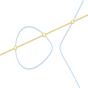
$$$y^2 \equiv x^3 + 2x + 3 \pmod{97}$ $$$P = (3, 6)$ and $$$Q = (80, 87)$ . 5. , $$$(a, b)$ and $$$(A, B)$ , . $$$(3, 3)$ and $$$(2, 0)$ , which allows us to calculate the logarithm as $$$x = (3 - 2)(0 - 3)^{-1} \bmod{5} = 3$ . And in fact, we did $$$Q = 3P$ .

In essence, we take a pseudo-random sequence of pairs. $$( a , b ) together with the corresponding sequence of points$(a, b)$$$$aP + bQ$ . Sequence of pairs $$( a , b ) may or may not be cyclic, but the sequence of points is exactly cyclic, because$(a, b)$$$$P$ and $$Q are generated from one base point, and from the property of subgroups we know that we cannot “escape” from a subgroup only by scalar multiplication and addition. Now we take two animals, a tortoise and a hare, and force to bypass the sequence from left to right. The turtle(the green dot in the image) is slow andreads every dot, one after the other; The hare(red dot) is fast andskips the dot at each step. After some time, the tortoise and the hare will find one point, but with different pairs of coefficients. Or, to put it in equations, the turtle will find a pair$Q$



$$( a , b ) , and the hare is a pair$(a, b)$$$( A , b ) such that$(A, B)$$$$aP + bQ = AP + BQ$ .

If a random sequence is determined through an algorithm (and not stored statically), it is easy to see that the principle of operation requires all $$$O (\ log n)$ space. The calculation of the asymptotic time complexity is not so simple, but we can construct a probabilistic proof showing that thetime complexity is equal to $$$O(\sqrt{n}$ )as we said.

Experimenting with Pollard ρ

I created a Python script that calculates discrete logarithms using the Pollard ρ-algorithm. This is not a realization of the original Pollard ρ, but a small variation of it (I used a more efficient way of generating a pseudo-random sequence of pairs). The script has useful comments, so read it if you are interested in the details of the algorithm.

This script, like the baby-step giant-step, works for small curves and creates the same output.

Ro Pollard in practice

We said that the baby-step giant-step cannot be used in practice because of the huge memory requirements. On the other hand, the Pollard ro-algorithm requires very little memory. How practical is it?

In 1998, Certicom began a competition in computing discrete logarithms on elliptic curves with a bit length from 109 to 369. To date, only curves with a length of 109 bits have been successfully cracked . The last successful attempt was made in 2004. We quote Wikipedia :

The award was presented on April 8, 2004 to approximately 2,600 people who were represented by Chris Monico. They also used a variant of the Pollard parallelized po-algorithm, the calculations for which took 17 months of calendar time.

As we have said, prime192v1this is one of the “smallest” elliptic curves. We also said that ρ Pollard has a time complexity$$$O(\sqrt{n})$ .If we used the same technique as Chris Monico (same algorithm, same equipment and number of machines), how much would the logarithm calculation take for prime192v1?

$$

$$17\ \text{}\ \times \frac{\sqrt{2^{192}}}{\sqrt{2^{109}}} \approx 5 \cdot 10^{13}\ \text{}$$

The result speaks for itself and makes it clear how difficult it is to crack the discrete logarithm using such techniques.

Compare ρ Pollard and Baby-step giant-step

I decided to combine the baby-step giant-step script , the Pollard ro script and the brute force script into the fourth script to compare their performance.

This fourth script calculates all logarithms for all points on the “small” curve using different algorithms and reports how long it took:

 Curve order: 10331 Using bruteforce Computing all logarithms: 100.00% done Took 2m 31s (5193 steps on average) Using babygiantstep Computing all logarithms: 100.00% done Took 0m 6s (152 steps on average) Using pollardsrho Computing all logarithms: 100.00% done Took 0m 21s (138 steps on average) 

As you might expect, the brute force method is monstrously slow compared to the other two. Baby-step giant-step is faster, and Pollard's po-algorithm is more than three times slower than baby-step giant-step (although it uses much less memory and fewer steps on average).

Look also at the number of steps: on average, it took 5,193 steps to calculate each logarithm using the brute force method. 5193 is very close to 10331/2 (half the order of the curve). Baby-step giant-steps and Pollard ro used 152 steps and 138 steps, respectively. These two numbers are very close to the square root of 10331 (101.64).

Further reasoning

In the discussion of these algorithms, I used a lot of numbers. When reading them, it is important to be careful: the algorithms in many aspects can be highly optimized. Equipment may improve. You can create specialized equipment.

If today the approach seems impractical, it does not mean that it cannot be improved. It also does not mean that there are no other, better approaches (do not forget that we have no proof of the complexity of the discrete logarithm problem).

Shore Algorithm

If modern techniques are not applicable, then what about the techniques of the near future? The situation is becoming more and more disturbing: there is already a quantum algorithm capable of computing discrete logarithms in polynomial time: Shor's algorithm with time complexity$$O ( ( log n ) 3 ) and spatial complexity$O((\log n)^3)$$$$O (\ log n)$ .

The effectiveness of quantum algorithms is a superposition of the state. In classical computers, memory cells (i.e., bits) can be 1 or 0. There are no intermediate states between them. On the other hand, the memory cells of quantum computers (qubits) are subject to the principle of uncertainty: as long as they are not measured, they do not have a fully defined state. The superposition of the state does not mean that each qubit can have the value 0 and 1 at the same time (as often written on the Internet). It means that when measuring a qubit, we have a certain probability to observe 0 and another probability to observe 1. The work of quantum algorithms consists in changing the probability of each qubit.

This oddity means that with a limited number of qubits we can simultaneously deal with a lot of possible input data at the same time. For example, we can tell a quantum computer that there is a number$$x evenly distributed between 0 and$x$$$$n - 1$ . This requires only $$log n qubits instead$\log n$$$$n \log n$ bit. Then we can order the quantum computer to perform scalar multiplication $$$xP$ . As a result, we obtain a superposition of states given by all points from $$$0P$ before $$( n - 1 ) P , that is, if we now measure all qubits, then we get one of the points from$(n - 1)P$$$$0P$ before $$( n - 1 ) P with probability$(n - 1)P$$$$1 / n$ .

I talked about this so that you understand the power of the superposition of states. Shor's algorithm does not work quite like that, in fact it is more complicated. It is complicated by the fact that although we can "simulate"$$n states at the same time, at some stage we will have to reduce this number of states to several, because at the output we need one number, not several (i.e., we need to know one logarithm, but not many likely erroneous logarithms).$n$

ECC and RSA

Now let's forget about quantum computing, which has not yet become a serious problem. I want to answer the following question: why bother with elliptic curves, if RSA and so works well?

A simple answer was given by NIST, presenting a table comparing the sizes of the RSA and ECC keys needed to obtain the same level of protection.

RSA key size (bits)	ECC key size (bits)
1024	160
2048	224
3072	256
7680	384
15360	521

Note that there is no linear relationship between the RSA and ECC key sizes (in other words: if we double the RSA key size, we do not need to double the ECC key size). The table tells us that ECC not only uses less memory, but also generates keys with signing in it much faster.

But why is this so? The answer is that the fastest algorithms for computing discrete algorithms over elliptic curves are the Pollard ρ-algorithm and the baby-step giant-step, and in the case of RSA there are faster algorithms. In particular, one of them is the general sieve of the numerical field.: An algorithm for factoring integers that can be used to compute discrete logarithms. The general sieve of the numerical field is by far the fastest algorithm for factoring integers.

All of this applies to other cryptosystems based on modular arithmetic, including DSA, Diffie-Hellman and El Gamal.

Hidden threats to the NSA

And now for the difficult part. Up to this point we have been discussing algorithms and mathematics. It is time to discuss people, and everything becomes more complicated.

If you remember, in the third part we said that some classes of elliptic curves are weak, so to solve the problem of obtaining reliable curves from dubious sources, we add a random seed value to the parameters of the domain of definition. And if you look at the standard NIST curves, you can see that they are testable random.

If you read the Wikipedia page on the principle "there is nothing in the sleeves, " you will notice that:

• MD5 random numbers are obtained from the sine of integers.
• Random numbers for Blowfish are obtained from the first numbers $$$\ pi$ .
• Random numbers for RC5 are obtained from $$e and the golden section.$e$

These numbers are random, because their numbers are evenly distributed. And they do not arouse suspicion, because they have a rationale.

Now the next question arises: where do the random generator values ​​for the NIST curves come from? Answer: unfortunately, we do not know. These values ​​have no justification.

Is it possible that NIST found a “significantly large” class of weak elliptic curves, tried various possible generator values, and found a vulnerable curve? I can not answer this question, but it is a natural and important question. We know that at least NIST has successfully standardized a vulnerable random number generator.(generator, which, oddly enough, is based on elliptic curves). Perhaps he successfully standardized and many weak elliptic curves? How to check it? Yes, nothing.

It is important to understand that “verifiable random” and “protected” are not synonymous. And no matter how difficult the logarithm task is or how long the keys are - if the algorithms are hacked, then we can’t do anything.

In this regard, RSA wins because it does not require special definition domain parameters that can be exploited. RSA (like other modular arithmetic systems) can be a good alternative if we cannot trust the authorities and if we cannot create our own definition domain parameters. And if you're curious, yes, TLS can use NIST curves. If you check in google, you will see that the connection uses ECDHE and ECDSA with a certificate based on prime256v1(it is the same secp256p1).

That's all!

Hope you enjoyed this article.I wanted to introduce you to the basic information, terminology and assumptions necessary to understand the current state of cryptography on elliptic curves. If I succeeded, now you can deal with existing ECC-based cryptosystems and expand your knowledge by reading deeper documentation. When writing this article I missed a lot of details and used simplified terminology, but I felt that otherwise you would not understand the information presented on the Internet. I believe that I managed to find a good compromise between simplicity and completeness of information.

However, it is worth noting that after reading only this article, you will not be able to implement ECC-based secure cryptosystems: security requires knowledge of many subtle, but important details. Recall the requirements for the Smart attack and the Sony error — these are two examples of how unsafe algorithms can be created and how easily they can be exploited.

So, if you are interested in plunging deeper into the world of ECC, then where do you start?

First, for the time being we saw Weierstrass curves over simple fields, but you should know that there are other types of curves and fields, namely:

• Koblitz curves over binary fields. These are elliptic curves in shape.$$$y^2 + xy = x^3 + ax^2 + 1$ (Where $$$a$ — 0 1) , $$$2^m$ ( $$$m$ — ). .
  
  nistk163 , nistk283 nistk571 ( , 163, 283 571 ).
• . $$$x^2 + xy = x^3 + x^2 + b$ (Where $$$b$ — , ). , . nistb163 , nistb283 nistb571 .
  
  , , , .
• $$$x^2 + y^2 = 1 + d x^2 y^2$ (Where $$$d$ — 0 1). , , , , ( $$$P \ne Q$ , $$$P = Q$ , $$$P = -Q$ , ...). (side-channel attack), , , .
  
  ( 2007 ), , Certicom NIST, .
• Curve25519 and Ed25519 are two special elliptic curves created for the ECDH and the ECDSA variant, respectively. Like the Edwards curves, these two curves are quick and help defend against attacks through third-party channels. Like Edwards curves, these two curves have not yet been standardized and are not used in popular software (with the exception of OpenSSH, which supports Ed25519 key pairs since 2014).

If you are interested in the details of the ECC implementation, I suggest you read the OpenSSL and GnuTLS sources .

And finally, if you are interested in the mathematical details, and not the safety and efficiency of algorithms, then you need to know the following:

• Elliptic curves are algebraic varieties of genus 1 .
• Infinitely distant points are studied in projective geometry . They can be represented using homogeneous coordinates (although most of the properties of projective geometry are not needed for cryptography on elliptic curves).

And do not forget to study the final fields along with field theory .

If you are interested in this topic, you should look for such keywords.

This article officially ends. Thanks for all the friendly comments, tweets and letters. Many asked if I would write other articles about related topics. My answer: maybe. You can send your suggestions, but I promise nothing.