Visualization of latent semantic analysis results using Python tools
Formulation of the problem
Semantic (semantic) text analysis is one of the key problems of both the theory of creating artificial intelligence systems relating to the processing of natural language (Natural Language Processing, NLP) and computational linguistics. The results of semantic analysis can be used to solve problems in such areas as, for example, psychiatry (to diagnose patients), political science (prediction of election results), trade (analysis of the demand for certain goods based on comments on this product), philology (analysis of copyright texts ), search engines, automatic translation systems. Google search engine is fully built on semantic analysis.
Visualization of the results of semantic analysis is an important stage of its implementation because it can provide quick and effective decision-making based on the results of the analysis.
Analysis of publications in the network on latent semantic analysis (LSA) shows that the visualization of the analysis results is given only in two publications [1,2] in the form of a two coordinate graph of the semantic space with plotted coordinates of words and documents. Such visualization does not allow to unambiguously identify groups of close documents and to assess the level of their semantic connection by the words belonging to the documents. Although in my publication titled “Complete latent semantic analysis using Python tools” [1], an attempt was made to use cluster analysis of latent semantic analysis results, however, only cluster marks and centroid coordinates for groups of words and documents without visualization were identified.
')
Visualization of LSA results by cluster analysis
We present all the steps of the LSA, including visualization of the results by the clustering method:
- Stop words are excluded from the analyzed documents. These are words that occur in every text and do not carry a semantic load; they are, first of all, all unions, particles, prepositions, and many other words.
- From the analyzed documents it is necessary to filter the numbers, individual letters and punctuation marks.
- Delete the words that are found in all documents only once. This does not affect the final result, but greatly simplifies mathematical calculations.
- With all the words from the documents should be carried out the operation of stemming - getting the basis of the word.
- Create a frequency matrix indexable lov. In this matrix, the rows correspond to the indexed words, and the columns correspond to the documents. Each cell of the matrix must indicate how many times the word occurs in the corresponding document.
- The resulting frequency matrix should be normalized. The standard way to normalize the matrix TF-IDF [3].
- The next step is a singular decomposition of the resulting matrix. Singular decomposition [4]; - is a mathematical operation, decomposing the matrix into three components. Those. We represent the initial matrix M in the form:
M = U * W * V ^ t
where U and V ^ t are orthogonal matrices, and W is a diagonal matrix. Moreover, the diagonal elements of the matrix W are ordered in decreasing order. The diagonal elements of the matrix W are called singular numbers. - Discard the last columns of the matrix U and the last rows of the matrix V ^ t, leaving only the first 2. These are the X, Y coordinates of each word for the U matrix and the X, Y coordinates for each document in the V ^ t matrix, respectively. A decomposition of this type is called a two-dimensional singular decomposition.
- Discard the last columns of the matrix U and the last rows of the matrix V ^ t, leaving only the first 3. These are respectively the X, Y, Z coordinates of each word for the U matrix and the X, Y, Z coordinates for each document in the V ^ t matrix. The decomposition of this type is called the three-dimensional singular decomposition.
- Preparation of source data in the form of nested lists of X, Y coordinates for two columns of the matrix U of words and two rows of the matrix of V ^ t documents.
- The construction of diagrams of Euclidean distances between the rows of two columns of the matrix U and the columns of two rows of the matrix V ^ t.
- Isolation of the number of clusters [5,6,7].
- Construction of diagrams and dendrograms.
- Preparation of source data in the form of nested lists of coordinates X, Y, Z for three columns of the matrix U of words and three rows of the matrix V ^ t of documents.
- The allocation of the number of clusters.
- Construction of diagrams and dendrograms.
- Comparison of cluster analysis results for two-dimensional and three-dimensional singular decomposition of the normalized frequency matrix of words and documents.
To implement the above steps, a special program was developed in which the same test set of documents was used for comparison as in the publication [2].
The program for visualizing the results of LSA
The result of the program
The first 2 columns of the orthogonal matrix U of words
wikileaks [-0.0741 0.0991]
arrest [-0.023 0.0592]
British [-0.023 0.0592]
handed [-0.0582 -0.5008]
Nobel [-0.0582 -0.5008]
founder [-0.0804 0.1143]
polits [-0.0337 0.0846]
Prem [-0.0582 -0.5008]
proto [-0.5954 0.0695]
countries [-0.3261 -0.169]
court [-0.3965 0.1488]
usa [-0.5954 0.0695]
Ceremony [-0.055 -0.3875]
The first 2 rows of the orthogonal matrix of Vt documents
[[0.0513 0.6952 0.1338 0.045 0.0596 0.2102 0.6644 0.0426 0.0566]
[-0.1038 -0.1495 0.5166 -0.0913 0.5742 -0.1371 0.0155 -0.0987 0.5773]]
The first 3 columns of the orthogonal matrix U of words
wikileaks [-0.0741 0.0991 -0.4372]
arrest [-0.023 0.0592 -0.3241]
British [-0.023 0.0592 -0.3241]
handed [-0.0582 -0.5008 -0.1117]
Nobel [-0.0582 -0.5008 -0.1117]
founder [-0.0804 0.1143 -0.5185]
police [-0.0337 0.0846 -0.4596]
Prem [-0.0582 -0.5008 -0.1117]
proto [-0.5954 0.0695 0.1414]
countries [-0.3261 -0.169 0.0815]
court [-0.3965 0.1488 -0.1678]
United States [-0.5954 0.0695 0.1414]
Ceremony [-0.055 -0.3875 -0.0802]
The first 3 rows of the orthogonal matrix of Vt documents
[[0.0513 0.6952 0.1338 0.045 0.0596 0.2102 0.6644 0.0426 0.0566]
[-0.1038 -0.1495 0.5166 -0.0913 0.5742 -0.1371 0.0155 -0.0987 0.5773]
[0.5299 -0.0625 0.0797 0.4675 0.1314 0.3714 -0.1979 0.5271 0.1347]]
#!/usr/bin/env python # -*- coding: utf-8 -*- import numpy from numpy import * import nltk import scipy from nltk.corpus import brown from nltk.stem import SnowballStemmer from scipy.spatial.distance import pdist from scipy.cluster import hierarchy import matplotlib.pyplot as plt stemmer = SnowballStemmer('russian') stopwords=nltk.corpus.stopwords.words('russian') # docs =[ " WikiLeaks",# № 0 " , ",# №1 " 19 ",# №2 " Wikileaks ",# №3 " ",# №4 " Wikileaks",# №5 " ",# №6 " WikiLeaks, , ",# №7 " "# №8 ] word=nltk.word_tokenize((' ').join(docs))# n=[stemmer.stem(w).lower() for w in word if len(w) >1 and w.isalpha()]# stopword=[stemmer.stem(w).lower() for w in stopwords]# - fdist=nltk.FreqDist(n) t=fdist.hapaxes()# # d={};c=[] for i in range(0,len(docs)): word=nltk.word_tokenize(docs[i]) word_stem=[stemmer.stem(w).lower() for w in word if len(w)>1 and w.isalpha()] word_stop=[ w for w in word_stem if w not in stopword] words=[ w for w in word_stop if w not in t] for w in words: if w not in c: c.append(w) d[w]= [i] elif w in c: d[w]= d[w]+[i] a=len(c); b=len(docs) A = numpy.zeros([a,b]) c.sort() for i, k in enumerate(c): for j in d[k]: A[i,j] += 1 # TF-IDF wpd = sum(A, axis=0) dpw= sum(asarray(A > 0,'i'), axis=1) rows, cols = A.shape for i in range(rows): for j in range(cols): m=float(A[i,j])/wpd[j] n=log(float(cols) /dpw[i]) A[i,j] =round(n*m,2) # U, S,Vt = numpy.linalg.svd(A) rows, cols = U.shape for j in range(0,cols): for i in range(0,rows): U[i,j]=round(U[i,j],4) print(' 2 U ') for i, row in enumerate(U): print(c[i], row[0:2]) res1=-1*U[:,0:1]; res2=-1*U[:,1:2] data_word=[] for i in range(0,len(c)):# data_word.append([res1[i][0],res2[i][0]]) plt.figure() plt.subplot(221) dist = pdist(data_word, 'euclidean')# ( ) plt.hist(dist, 500, color='green', alpha=0.5)# Z = hierarchy.linkage(dist, method='average')# plt.subplot(222) hierarchy.dendrogram(Z, labels=c, color_threshold=.25, leaf_font_size=8, count_sort=True,orientation='right') print(' 2 Vt ') rows, cols = Vt.shape for j in range(0,cols): for i in range(0,rows): Vt[i,j]=round(Vt[i,j],4) print(-1*Vt[0:2, :]) res3=(-1*Vt[0:1, :]);res4=(-1*Vt[1:2, :]) data_docs=[];name_docs=[] for i in range(0,len(docs)): name_docs.append(str(i)) data_docs.append([res3[0][i],res4[0][i]]) plt.subplot(223) dist = pdist(data_docs, 'euclidean') plt.hist(dist, 500, color='green', alpha=0.5) Z = hierarchy.linkage(dist, method='average') plt.subplot(224) hierarchy.dendrogram(Z, labels=name_docs, color_threshold=.25, leaf_font_size=8, count_sort=True) #plt.show() print(' 3 U ') for i, row in enumerate(U): print(c[i], row[0:3]) res1=-1*U[:,0:1]; res2=-1*U[:,1:2];res3=-1*U[:,2:3] data_word_xyz=[] for i in range(0,len(c)): data_word_xyz.append([res1[i][0],res2[i][0],res3[i][0]]) plt.figure() plt.subplot(221) dist = pdist(data_word_xyz, 'euclidean')# ( ) plt.hist(dist, 500, color='green', alpha=0.5)# Z = hierarchy.linkage(dist, method='average')# plt.subplot(222) hierarchy.dendrogram(Z, labels=c, color_threshold=.25, leaf_font_size=8, count_sort=True,orientation='right') print(' 3 Vt ') rows, cols = Vt.shape for j in range(0,cols): for i in range(0,rows): Vt[i,j]=round(Vt[i,j],4) print(-1*Vt[0:3, :]) res3=(-1*Vt[0:1, :]);res4=(-1*Vt[1:2, :]);res5=(-1*Vt[2:3, :]) data_docs_xyz=[];name_docs_xyz=[] for i in range(0,len(docs)): name_docs_xyz.append(str(i)) data_docs_xyz.append([res3[0][i],res4[0][i],res5[0][i]]) plt.subplot(223) dist = pdist(data_docs_xyz, 'euclidean') plt.hist(dist, 500, color='green', alpha=0.5) Z = hierarchy.linkage(dist, method='average') plt.subplot(224) hierarchy.dendrogram(Z, labels=name_docs_xyz, color_threshold=.25, leaf_font_size=8, count_sort=True) plt.show() The result of the program
The first 2 columns of the orthogonal matrix U of words
wikileaks [-0.0741 0.0991]
arrest [-0.023 0.0592]
British [-0.023 0.0592]
handed [-0.0582 -0.5008]
Nobel [-0.0582 -0.5008]
founder [-0.0804 0.1143]
polits [-0.0337 0.0846]
Prem [-0.0582 -0.5008]
proto [-0.5954 0.0695]
countries [-0.3261 -0.169]
court [-0.3965 0.1488]
usa [-0.5954 0.0695]
Ceremony [-0.055 -0.3875]
The first 2 rows of the orthogonal matrix of Vt documents
[[0.0513 0.6952 0.1338 0.045 0.0596 0.2102 0.6644 0.0426 0.0566]
[-0.1038 -0.1495 0.5166 -0.0913 0.5742 -0.1371 0.0155 -0.0987 0.5773]]
The first 3 columns of the orthogonal matrix U of words
wikileaks [-0.0741 0.0991 -0.4372]
arrest [-0.023 0.0592 -0.3241]
British [-0.023 0.0592 -0.3241]
handed [-0.0582 -0.5008 -0.1117]
Nobel [-0.0582 -0.5008 -0.1117]
founder [-0.0804 0.1143 -0.5185]
police [-0.0337 0.0846 -0.4596]
Prem [-0.0582 -0.5008 -0.1117]
proto [-0.5954 0.0695 0.1414]
countries [-0.3261 -0.169 0.0815]
court [-0.3965 0.1488 -0.1678]
United States [-0.5954 0.0695 0.1414]
Ceremony [-0.055 -0.3875 -0.0802]
The first 3 rows of the orthogonal matrix of Vt documents
[[0.0513 0.6952 0.1338 0.045 0.0596 0.2102 0.6644 0.0426 0.0566]
[-0.1038 -0.1495 0.5166 -0.0913 0.5742 -0.1371 0.0155 -0.0987 0.5773]
[0.5299 -0.0625 0.0797 0.4675 0.1314 0.3714 -0.1979 0.5271 0.1347]]
Diagrams and dendrograms of two-dimensional singular decomposition of the normalized frequency matrix of words and documents.
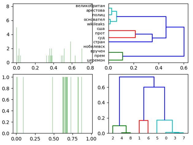
Obtained a clear visualization of the proximity of documents (see docs) and the belonging of words to documents.
Charts and dendrograms of the three-dimensional singular decomposition of the normalized frequency matrix of words and documents.
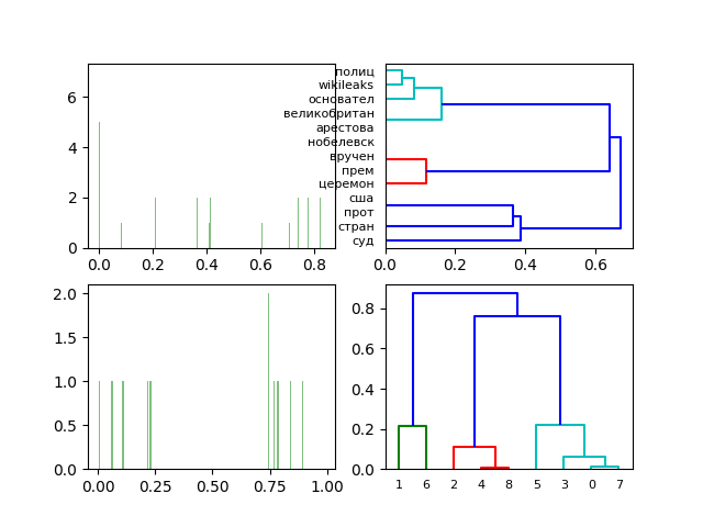
The transition to the three-dimensional singular decomposition of the normalized frequency matrix of words and documents for the given set of documents (see docs) does not qualitatively change the result of the LSA analysis.
findings
The given LSA visualization technique, in my opinion, is a successful addition to the LSA itself and deserves the attention of developers.
Thank you all for your attention!
Links
- Complete latent semantic analysis with Python tools.
- Latent semantic analysis and search in Python.
- TF-IDF-Wikipedia.
- Singular decomposition - Wikipedia.
- Visualization of cluster analysis in Python (hcluster and matplotlib modules).
- Hierarchical cluster analysis in the Python programming language.
- Algorithm k-means [Cluster analysis and Python].
Source: https://habr.com/ru/post/335668/
All Articles