Log it: the method of the logarithmic derivative in machine learning

The technique in question — the method of the logarithmic derivative — helps us do all sorts of things using the main property of the derivative of the logarithm. Best of all, this method has proven itself in solving stochastic optimization problems that we investigated earlier . Thanks to its application, we found a new way to obtain stochastic gradient estimates. We start with an example of using reception to determine the evaluation function.

Pretty mathematically.

Evaluation function (score function)

The method of the logarithmic derivative is the application of the rule for the gradient to the parameters θ of the logarithm of the function p (x; θ) :

$$$$ display $$ logθ log p (x; θ) = ∇θp (x; θ) / p (x; θ) $$ display $$

The application of the method turns out to be successful when the function p (x; θ) is a likelihood function , that is, the function f with parameters θ is the probability of a random variable x . In this particular case, the function

$$

$$∇θlogp (x; θ)$$

is called evaluative , and the right-hand side is a relation of evaluations. The evaluation function has a number of useful properties:

Basic operation for maximum likelihood estimation . Maximum likelihood is one of the main principles of machine learning used in generalized linear regression , in- depth training , nuclear machines , dimension reduction and tensor decompositions , etc. Evaluation is needed in all these tasks.

The expectation score is zero . Our first use of the logarithmic derivative method will show this:
')


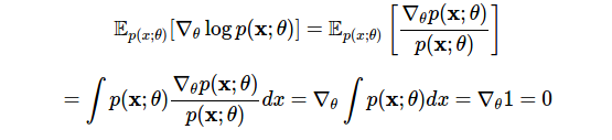
In the first line we applied the derived logarithm, and in the second line we changed the order of differentiation and integration. This identity detects the type of probabilistic flexibility we need: it allows you to subtract any term from a zero-expectation estimate, and the change will not affect the expected result (see below: control variables).

The variance of the estimate is the Fisher information used to determine the Cramer-Rao lower bound .



Now we can move in one boundary from the gradients of the logarithmic probability to the gradients of probability and back. However, the main evil character of today's post - the complex expected gradient from Method 4 - arises again. We can use our new power (the evaluation function) and find another clever evaluation solution for this class of problems.

Evaluation function evaluation unit

Our task is to calculate the gradient of the mathematical expectation of the function f :



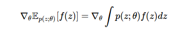
This is a frequently encountered machine learning problem, which is necessary for subsequent computation in variational derivation , the function of values ​​and the teaching of policies (strategies) in the learning process with reinforcement , the pricing of derivatives in financial engineering , inventory accounting in operations research, etc.

It is difficult to calculate this gradient, since the integral is usually unknown, and the parameters θ , with respect to which we calculate the gradient, have the distribution p (z; θ) . In addition, we may need to calculate this gradient for a non-differentiable function. Using the logarithmic derivative method and the properties of the estimation function, we can calculate this gradient in a more convenient way:



We derive this expression and consider its consequences for our optimization problem. For this purpose, we will use another frequently encountered method - the method of probability identity, according to which we multiply our expressions by 1 - the number formed by dividing the probability density by itself. Combining this method with the method of the logarithmic derivative, we get the evaluation unit of the evaluation function of the gradient:



In these four lines, we performed many operations. In the first line, we replaced the derivative with an integral. In the second, we applied our probabilistic method, which allowed us to form the coefficient of estimation. Using the logarithmic derivative, we replaced this coefficient with the gradient of the logarithmic probability in the third row. This gives us the desired stochastic estimate in the fourth line, which we calculated by the Monte Carlo method, taking a sample from p (z) and then calculating the weighted gradient term.

This is an unbiased gradient estimate . Our assumptions in this process were simple:

• The replacement of integration by differentiation is valid. This is difficult to show in general terms, but the replacement itself usually causes no problems. We can confirm the correctness of this technique, referring to the Leibniz formula and the analysis given here [ 1 ].
• The function f (z) should not be differentiable. So we can evaluate it or observe changes in values ​​for a given z .
• Obtaining samples from the distribution of p (z) is not difficult, since it is necessary to estimate the integral by the Monte Carlo method.

Like many of our other techniques, the path we have chosen here has already been covered in many other research areas, and each area already has its own term, a history of method development and a range of tasks related to the formulation of the problem. Here are some examples:

1. Assessment function evaluation unit (Score function estimator)

Our conclusion allowed us to convert the waiting gradient to the expectation of the evaluation function

$$

$$∇θlogp (z; θ),$$

which makes it convenient for designating such estimates as blocks of the evaluation function [ 2 ]. This is a fairly common term, and I prefer to use it.

Many insightful observations and a number of historically important developments on the topic are presented in the paper entitled " Optimization and sensitivity analysis of computer simulation models using the evaluation function method ".

2. Likelihood ratio methods

One of the main popularizers of this class of evaluation was P.V. Glynn [ 3 ]. He interprets the attitude of evaluation

$$$$ display $$ ∇θp (z; θ) / p (z; θ) $$ display $$

as likelihood ratio and describes evaluation units as likelihood ratio methods. I believe that this is a somewhat non-standard use of the term "likelihood ratio". It usually represents the ratio of the same function with different parameters, and not the ratio of different functions with the same parameter. Therefore, I prefer the term “Evaluation function evaluation unit”.

Many authors, and in particular, for example, Michael Foo [ 4 ], speak about methods of likelihood ratio and estimation (LR / SF). The most important work on the topic: "The estimated ratio of the likelihood coefficient for stochastic systems ", where Glynn explains in detail the most important properties of dispersion, and Michael Fu's Grade Evaluation .

3. Automated variation output

Variational derivation transforms difficult-to-solve integrals arising in Bayesian analysis into problems for stochastic optimization. It is not surprising that in this area there are also evaluation units for estimating functions known under different terms: variational stochastic search , automatic variational inference , variational inference on the black box model , neural variational inference — these are just a few of which I know.

4. Remuneration and strategy gradients

To solve reinforcement learning problems , we can compare the function f with the reward received from the environment, the distribution of p (z; θ) with the policy, and the evaluation with the gradient of the policy or, in some cases, with the characteristic possible choice (characteristic eligibility).

Intuitively, this can be explained as follows: any policy gradients that correspond to high remuneration receive large weights due to reinforcement from the evaluation unit. Consequently, the evaluation unit is called REINFORCE (REINFORCEMENT) [ 5 ] and this generalization at the moment forms the strategy (policy) gradient theorem .

Control variables

To do this Monte Carlo estimation effectively, we need to make its variance as small as possible. Otherwise, there will be no benefit from the gradient. To achieve greater control of dispersion is possible through the use of a modified estimate:



where the new term λ is called the control variable , widely used to reduce the variance in Monte-Carlo estimates. The control variable is any additional term added to the estimate that has a zero mean value. Such variables can be entered at any stage, as they do not affect expectations. Control variables affect variance. The main problem with the use of estimates is the choice of the reference variable. The easiest way is to use a constant parameter, but there are other methods: reasonable sampling schemes (for example, antithetical or stratified ), delta methods or adaptive constant parameters. One of the most comprehensive discussions of the sources of dispersion and methods for reducing dispersion is given in this book by P. Glaserman [ 6 ]

Groups of stochastic evaluation systems

Compare today's estimate with the one we derived using the linear derivative method in method 4 .



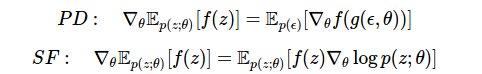
Here we have two effective approaches. We can:

• differentiate the function f using linear derivatives if the function is differentiable, or
• Differentiate the density of p (z) using the estimation function.

There are other ways to create stochastic gradient estimates, but these two are the most common. They can be easily combined, which allows us to use the most suitable estimate (providing the lowest variance) at different stages of our calculations. This problem can be solved, in particular, by using a stochastic computational graph .

Conclusion

The method of the logarithmic derivative allows us to alternate the normalized probability and logarithmically probability representations of distributions. It constitutes the basis for the determination of the evaluation function, and serves as a method for the most plausible evaluation and important asymptotic analysis, which have formed most of our statistical knowledge. It is important to note that this method can be used to assess the general-purpose gradient in solving stochastic optimization problems that underlie many important machine learning problems that we currently face. Monte Carlo gradient estimates are necessary for the genuinely universal machine learning to which we aspire. For this, it is important to understand the patterns and methods underlying such an assessment.

---