Planetary landscape
It is difficult to argue that the landscape is an integral part of most computer games in open spaces. The traditional method of implementing the change in the surface surrounding the player’s surface is the following: we take the mesh (Mesh), which is the plane, and for each primitive in this grid, we displace along the normal to this plane by a specific value for this primitive. In simple terms, we have a 256-by-256-pixel single-channel texture and a plane grid. For each primitive, by its coordinates on the plane, we take the value from the texture. Now we simply shift the coordinates of the primitive along the normal to the plane by the obtained value (Fig. 1)
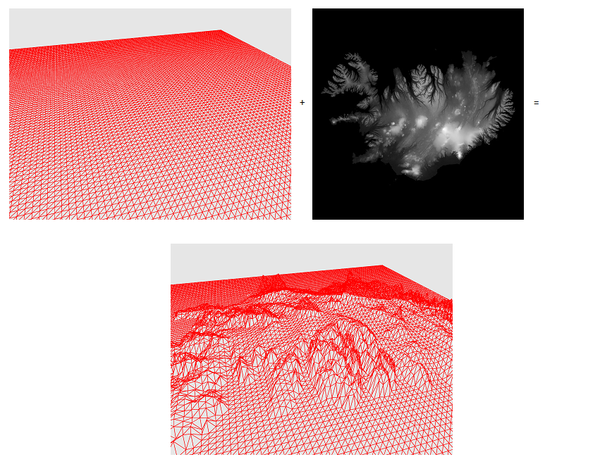
Fig.1 elevation map + plane = landscape
Why does this work? If we imagine that the player is on the surface of the sphere, and the radius of this sphere is extremely large relative to the size of the player, then the curvature of the surface can be neglected and the plane can be used. But what if we do not neglect the fact that we are on a sphere? I want to share my experience in building such landscapes with the reader in this article.
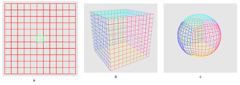
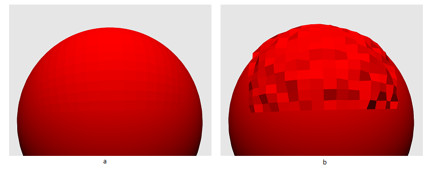
Obviously, it is not reasonable to build a landscape at once for the whole sphere - most of it will not be visible. Therefore, we need to create a certain minimum area of space - a certain primitive, of which the relief of the visible part of the sphere will consist. I will call it a sector. How do we get it? So look at fig.2a. The green box is our sector. Next, we construct six grids, each of which is a cube face (Fig. 2b). Now let's normalize the coordinates of the primitives that form the grids (Fig. 2c).
')
Pic2
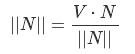
As a result, we got a cube projected onto a sphere, where the sector is the area on one of its faces. Why does this work? Consider an arbitrary point on the grid as a vector from the origin. What is vector normalization? This is a transformation of a given vector into a vector in the same direction, but with a unit length. The process is as follows: first we find the length of the vector in the Euclidean metric according to the Pythagorean theorem

Then we divide each of the vector components into this value.

Now we ask ourselves what is a sphere? A sphere is a set of points equidistant from a given point. The parametric sphere equation looks like this.
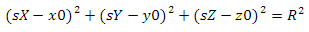
where x0, y0, z0 are the coordinates of the center of the sphere, and R is its radius. In our case, the center of the sphere is the origin, and the radius is one. Substitute the known values and take the root of the two parts of the equation. It turns out the following

Literally, the last transformation tells us the following: “In order to belong to a sphere, the vector length must be equal to one”. This we have achieved normalization.
What if the sphere has an arbitrary center and radius? Find the point that belongs to her by using the following equation
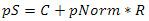
where pS is a point on the sphere, C is the center of the sphere, pNorm is the previously normalized vector and R is the radius of the sphere. In simple words, the following happens here: “we move from the center of the sphere towards the point on the grid at a distance R”. Since each vector has a unit length, in the end, all points are equidistant from the center of the sphere at a distance of its radius, which makes the equation of the sphere true.
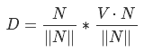
We need to get a group of sectors that are potentially visible from the viewpoint. But how to do that? Suppose we have a sphere with center at some point. We also have a sector that is located on a sphere and a point P located in the space near the sphere. Now we construct two vectors - one directed from the center of the sphere to the center of the sector, the other from the center of the sphere to the point of view. Look at Figure 3 - a sector can only be seen if the absolute value of the angle between these vectors is less than 90 degrees.
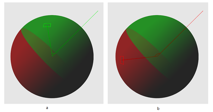
Fig.3 a - angle less than 90 - the sector is potentially visible. b - angle greater than 90 - sector is not visible
How to get this angle? To do this, use the scalar product of vectors. For the three-dimensional case, it is calculated as:

Scalar product has a distribution property:

Earlier, we defined the vector length equation - now we can say that the length of the vector is equal to the root of the scalar product of this vector itself. Or vice versa - the scalar product of the vector itself is equal to the square of its length.
Now let's turn to the law of cosines. One of his two formulations looks like this (Fig. 4):

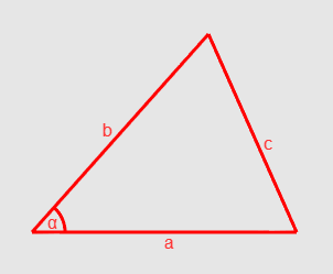
Fig.4 cosine law
If we take the lengths of our vectors as a and b, then the angle alfa is what we are looking for. But how do we get value with? See: if we take a from b, then we get a vector directed from a to b, and since the vector is characterized only by direction and length, then we can graphically arrange its beginning at the end of vector a. From this, we can say that c is equal to the length of the vector b - a. So we did
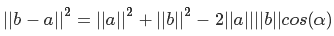
Express the squares of lengths as scalar products

open brackets using the distribution property

a little shorten

and finally, by dividing both equations of the equation by minus two, we get
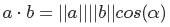
This is another property of the scalar product. In our case, we need to normalize the vectors so that their lengths are equal to one. We don’t need to calculate the angle - the cosine value is enough. If it is less than zero, then we can safely say that we are not interested in this sector.
It's time to think about how to draw primitives. As I said earlier, the sector is the main component in our scheme, so for each potentially visible sector we will draw a grid, the primitives of which will form the landscape. Each of its cells can be displayed using two triangles. Due to the fact that each cell has adjacent faces, the values of most triangle vertices are repeated for two or more cells. Not to duplicate the data in the vertex buffer, fill the index buffer. If indices are used, then with their help the graphic pipeline determines which primitive in the vertex buffer to process. (pic.5) The topology I chose is a triangle list (D3D11_PRIMITIVE_TOPOLOGY_TRIANGLELIST)

Fig.5 Visual display of indexes and primitives
Creating a separate vertex buffer for each sector is too expensive. It is much more efficient to use one buffer with coordinates in the grid space, that is, x is a column and y is a row. But how to get a point on the sphere from them? A sector is a square area with a beginning at a certain point S. All sectors have the same length of the face - let's call it SLen. The grid covers the entire area of the sector and also has the same number of rows and columns, so we can build the following equation to find the length of the cell face.
where CLen is the length of the cell face, MSize is the number of rows or columns of the grid. We divide both parts by MSize and get CLen

We go further. The space of the face of the cube to which the sector belongs can be expressed as a linear combination of two vectors of unit length — we call them V1 and V2. We have the following equation (see fig. 6)
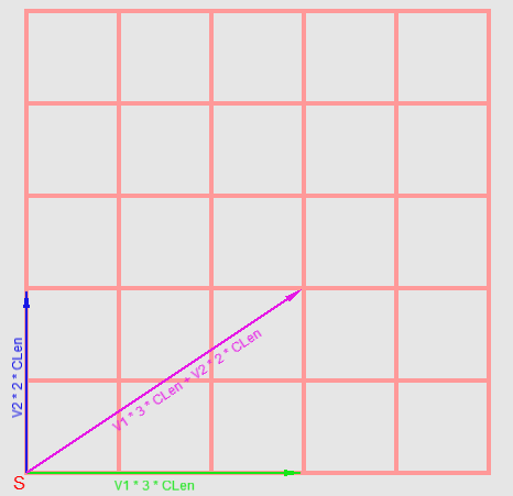
Fig.6 A visual representation of the formation of a point on the grid
to get a point on a sphere, we use the equation derived earlier
All that we have achieved by this moment is not very similar to the landscape. It's time to add what will make it so - the difference in height. Let's imagine that we have a sphere of unit radius with center at the origin of coordinates, as well as a set of points {P0, P1, P2 ... PN}, which are located on this sphere. Each of these points can be represented as a unit vector from the origin. Now imagine that we have a set of values, each of which is the length of a particular vector (Fig. 7).
I will store these values in a two-dimensional texture. We need to find the relationship between the coordinates of the pixel texture and the vector-point on the sphere. Let's get started
In addition to Cartesian, a point on a sphere can also be described using a spherical coordinate system. In this case, its coordinates will consist of three elements: the azimuth angle, the polar angle, and the value of the shortest distance from the origin to the point. The azimuth angle is the angle between the X axis and the projection of the ray from the origin to a point on the XZ plane. It can take values from zero to 360 degrees. Polar angle - the angle between the Y axis and the ray from the origin to the point. It can also be called zenith or normal. Accepts values from zero to 180 degrees. (see figure 8)
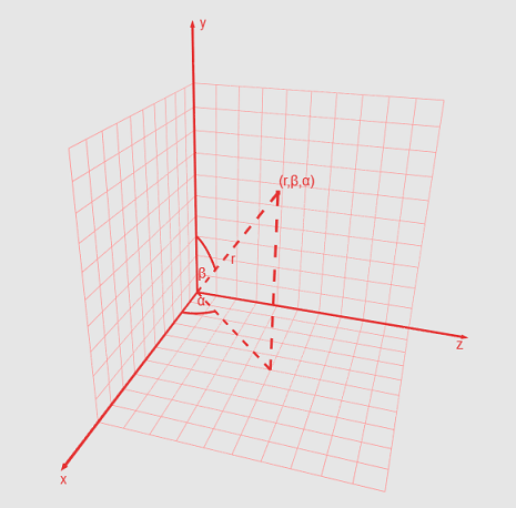
Fig.8 Spherical coordinates
To go from a Cartesian system to a spherical, I use the following equations (I believe that the Y axis is pointing up):

where d is the distance to the point, a is the polar angle, b is the azimuth angle. The parameter d can also be described as “the length of the vector from the origin to the point” (as can be seen from the equation). If we use normalized coordinates, we can avoid division when finding the polar angle. Actually, why do we need these corners? Dividing each of them into its maximum range, we obtain coefficients from zero to one and with their help we will select the texture from the shader. When obtaining the coefficient for the polar angle, it is necessary to take into account the quarter in which the angle is located. "But the value of the expression z / x is not defined when x is equal to zero" - you say. I will say more: when z equals zero, the angle will be zero regardless of the value of x.
Let's add some special cases for these values. We have normalized coordinates (normal) - we add several conditions: if the X value of the normal is zero and the Z value is greater than zero, then the coefficient is 0.25, if X is zero and Z is less than zero, then it will be 0.75. If the value of Z is zero and X is less than zero, then in this case the coefficient will be equal to 0.5. All this is easy to check on the circumference. But what to do if Z is zero and X is greater than zero - in this case, both 0 and 1 will be correct? Imagine that we chose 1 — well, let's take a sector with a minimum azimuth angle of 0 and a maximum angle of 90 degrees. Now consider the first three vertices in the first row of the grid that displays this sector. For the first vertex, we met the condition and set the textural coordinate of X to 1. It is obvious that for the next two vertices this condition will not be fulfilled - the angles for them are in the first quarter and as a result we get something like this - (1.0, 0.05, 0.1). But for a sector with angles from 270 to 360 for the last three vertices in the same line, everything will be correct - the condition for the last vertex will work, and we will get a set (0.9, 0.95, 1.0). If we choose zero as the result, we get sets (0.0, 0.05, 0.1) and (0.9, 0.95, 0.0) - in any case, this will lead to quite noticeable distortions of the surface. So let's apply the following. Take the center of the sector, then normalize its center, thereby moving it onto the sphere. Now we calculate the scalar product of the normalized center by the vector (0, 0, 1). Formally speaking, this vector is normal to the XY plane, and by calculating its scalar product with the normalized vector of the center of the sector, we can understand which side of the plane the center is from. If it is less than zero, then the sector is behind the plane and we need the value 1. If the scalar product is greater than zero, then the sector is in front of the plane and therefore the boundary value is 0. (see Fig.9)

Fig.9 The problem of choosing between 0 and 1 for texture coordinates
Here is the code for obtaining texture coordinates from spherical. Please note that because of the error in the calculations, we cannot check the values of the normal for equality to zero, instead we must compare their absolute values with a certain threshold value (for example, 0.001)
I will give an intermediate version of the vertex shader
In order to realize the dependence of the landscape color on lighting, we will use the following equation:

Where I is the color of the point, Ld is the color of the light source, Kd is the color of the material of the illuminated surface, a is the angle between the vector of the source and the normal to the illuminated surface. This is a special case of the Lambert cosine law. Let's see what is here and why. By multiplying Ld by Kd is meant componentwise color multiplication, that is (Ld.r * Kd.r, Ld.g * Kd.g, Ld.b * Kd.b). It may be easier to understand the meaning if we imagine the following situation: suppose we want to illuminate an object with a green light source, so we expect the color of the object to be in gradations of green. The result (0 * Kd.r, 1 * Kd.g, 0 * Kd.b) gives (0, Kd.g, 0) - exactly what we need. We go further. As stated earlier, the cosine of the angle between normalized vectors is their scalar product. Let's look at its maximum and minimum value from our point of view. If the cosine of the angle between the vectors is 1, then this angle is 0 - therefore, both vectors are collinear (lie on the same line).
The same is true for the cosine value of -1, only in this case the vectors point in opposite directions. It turns out, the closer the normal vector and the vector to the light source to the state of collinearity - the higher the luminance factor of the surface to which the normal belongs. It is also assumed that the surface cannot be illuminated if its normal points in the direction opposite to the direction to the source — that is why I use only positive cosine values.
I use a parallel source, so its position can be neglected. The only thing that needs to be taken into account is that we use a vector to the light source. That is, if the direction of the rays is (1.0, -1.0, 0) - we need to use the vector (-1.0, 1.0, 0). The only thing that is difficult for us is the normal vector. It is easy to calculate the normal to the plane - we need to produce the vector product of two vectors that describe it. It is important to remember that the vector product is anticommutative - you need to take into account the order of the factors. In our case, we can obtain the normal to the triangle, knowing the coordinates of its vertices in the space of the grid, as follows (Note that I do not take into account the boundary cases for px and py)
But that is not all. Most vertices of the grid belong immediately to four planes. To get an acceptable result, you need to calculate the average normal as follows:
Implementing this method on a GPU is quite expensive - we need two steps to calculate the normals and average them. In addition, the efficiency leaves much to be desired. Based on this, I chose another way - to use the normal map. (Fig.10)
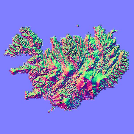
Pic.10 Normal map
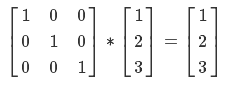
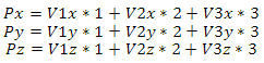
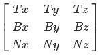
The principle of working with it is the same as with the height map - we transform the spherical coordinates of the grid vertex into textural coordinates and make a selection. Only we will not be able to use this data directly - after all, we work with the sphere, and the vertex has its own normal, which must be taken into account. Therefore, we will use the data of the normal map as the coordinates of the TBN basis. What is a basis? Here is an example. Imagine that you are an astronaut and are sitting on a beacon somewhere in space. You receive a message from the MCC: “You need to move from the beacon 1 meter to the left, 2 meters up and 3 meters ahead.” How can this be mathematically expressed? (1, 0, 0) * 1 + (0, 1, 0) * 2 + (0, 0, 1) * 3 = (1,2,3). In matrix form, this equation can be expressed as:
Now imagine that you are also sitting on the beacon, only now they write to you from the MCC: “we sent you direction vectors there - you have to move 1 meter along the first vector, 2 meters along the second and 3 along the third”. The equation for the new coordinates will be:
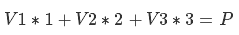
component entry is as follows:
Or in matrix form:

so, the matrix with the vectors V1, V2 and V3 is the basis, and the vector (1,2,3) is the coordinates in the space of this basis.
Imagine now that you have a set of vectors (basis M) and you know where you are relative to the beacon (point P). You need to know your coordinates in the space of this base - how much you need to move along these vectors to be in the same place. Imagine the required coordinates (X)

If P, M and X were numbers, we would simply divide both sides of the equation into M, but alas ... Let's go the other way - according to the property of the inverse matrix
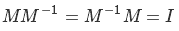
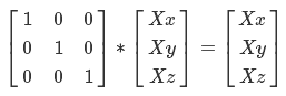
where I is the identity matrix. In our case, it looks like this.

What does this give us? Try multiplying this matrix by X and you will get
It is also necessary to clarify that the multiplication of matrices has the property of associativity

We can legitimately consider the vector as a 3 on 1 matrix.
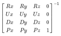
Considering the above, we can conclude that in order to get X in the right side of the equation, we need to multiply both sides in the correct order by the inverse M matrix

We will need this result in the future.
Now back to our problem. I will use an orthonormal basis, which means that V1, V2 and V3 are orthogonal with respect to each other (form an angle of 90 degrees) and have a unit length. The tangent vector will act as V1, V2 - bitangent vector, V3 - normal. In the traditional DirectX transposed form, the matrix looks like this:
where T is the tangent vector, B is the bitangent vector and N is the normal. Let's find them. With the normal, the easiest thing to do is essentially the normalized coordinates of a point. Bitangent vector is equal to the vector product of the normal and tangent vector. The hardest thing to do is with the tangent vector. It is equal to the direction of the tangent to the circle at the point. Let's break this down. First we find the coordinates of a point on the unit circle in the XZ plane for some angle a

The direction of the tangent to the circle at this point can be found in two ways. The vector to the point on the circle and the tangent vector are orthogonal — therefore, since the sin and cos functions are periodic, we can simply add pi / 2 to the angle a and obtain the desired direction. According to the bias property on pi / 2:
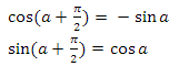
we have the following vector:

We can also use differentiation - see Appendix 3 for more details. Thus, in Figure 11 you can see a sphere, for each vertex of which a basis is built. Blue vectors are normals, red tangent vectors, green bitangent vectors.

Fig.11 Sphere with TBN bases at each vertex. Red - tangent vectors, green - bitangent vectors, blue vectors - normals
With the base figured out - now let's get the normal map. To do this, use the Sobel filter. The Sobel filter computes the gradient of the brightness of the image at each point (roughly speaking, the vector of brightness change). The principle of the filter is that you need to apply a certain matrix of values, which is called the "Core", to each pixel and its neighbors within the dimension of this matrix. Suppose that we process pixel P with the K kernel. If it is not on the border of the image, then it has eight neighbors — the left top, top, right top, and so on. We call them tl, t, tb, l, r, bl, b, br. So, the application of the K kernel to this pixel is as follows:
Pn = tl * K (0, 0) + t * K (0,1) + tb * K (0,2) +
& nbsp & nbsp & nbsp & nbsp & nbsp & nbsp & nbsp & nbsp & nbsp & nbspl * K (1, 0) + P * K (1,1) + r * K (1,2) +
& nbsp & nbsp & nbsp & nbsp & nbsp & nbsp & nbsp & nbsp & nbsp & nbspbl * K (2, 0) + b * K (2.1) + br * K (2.2)
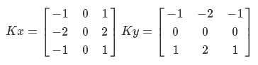
This process is called "convolution." The Sobel filter uses two cores to compute the gradient vertically and horizontally. Denote them as Kx and K:
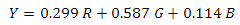
The basis is - you can begin to implement. First we need to calculate the pixel brightness. I use the conversion from the RGB color model to the YUV model for the PAL system:
But since our image is originally in grayscale, this stage can be skipped. Now we need to “collapse” the original image with the Kx and Ky cores. So we get the X and Y components of the gradient. The value of the normal of this vector may also be very useful - we will not use it, but images containing normalized values of the normal of the gradient have several useful applications. By normalization, I mean the following equation

where V is the value that we normalize, Vmin and Vmax are the range of these values. In our case, the minimum and maximum values are tracked during the generation process. Here is an example of the implementation of the Sobel filter:
I must say that the Sobel filter has the property of linear separability, so this method can be optimized.
The difficult part is over - it remains to record the X and Y coordinates of the gradient direction in the R and G channels of the pixels of the normal map. For the Z coordinates, I use a unit. I also use a three-dimensional vector of coefficients to adjust these values. The following is an example of generating a normal map with comments:
Now I will give an example of using the normal map in the shader:
Well, now our landscape is lit! You can fly to the moon - we zaguraem height map, set the color of the material, load the sectors, set the grid size to {16, 16} and ... Yes, something is not enough - put it on {256, 256} - oh, something slows down , and why high detail on distant sectors? Moreover, the closer the observer to the planet, the smaller sectors he can see. Yes ... we still have a lot of work to do! Let's first figure out how to cut off the extra sectors. The determining value here will be the height of the observer from the surface of the planet - the higher it is, the more sectors it can see (Figure 12)
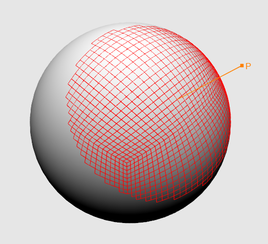
Fig.12. Dependence of the height of the observer on the number of sectors being processed.
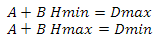
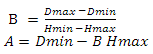
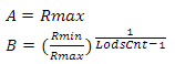
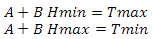
We find the height as follows: we construct the vector from the observer’s position to the center of the sphere, calculate its length and subtract the value of the radius of the sphere from it. Earlier, I said that if the scalar product of the vector on the observer and the vector on the center of the sector is less than zero, then this sector does not interest us - now instead of zero we will use a value linearly dependent on height. First let's define the variables - so we will have the minimum and maximum values of the scalar product and the minimum and maximum values of the height. Construct the following system of equations
Now we express A in the second equation
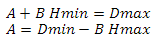
substitute A from the second equation into the first
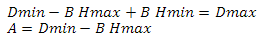
express B from the first equation
we substitute B from the first equation into the second
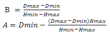
Now we will substitute variables in function

and get
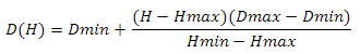
Where Hmin and Hmax are the minimum and maximum heights, Dmin and Dmax are the minimum and maximum values of the scalar product. This problem can be solved differently - see Appendix 4.
Now you need to understand the levels of detail. Each of them will determine the region of the value of the scalar product. In pseudocode, the process of determining whether a sector belongs to a certain level looks like this:
We need to calculate the range for each level. First, we construct a system of two equations
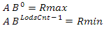
deciding it, we get
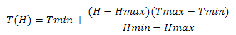
Using these coefficients, we define the function

where Rmax is the domain of the scalar product (D (H) - Dmin), Rmin is the minimum domain defined by the level. I use the value of 0.01. Now we need to subtract the result from Dmax

C using this function, we obtain areas for all levels. Here is an example:
Now we can determine to which level of detail the sector belongs (Fig. 13).

Fig.13 Color differentiation of sectors according to levels of detail
Next you need to deal with the size of the grid. It will be very expensive to store your grid for each level - it is much more efficient to change the detail of one grid on the fly using tessellation. To do this, in addition to the above-vertex and pixel ones, we also need to implement hull and domain shaders. In the Hull shader, the main task is to prepare control points. It consists of two parts - the main function and the function that calculates the parameters of the control point. Be sure to specify values for the following attributes:
See, the main work is done in GetPatchData (). Her task is to establish the tessellation factor. We will talk about it later, now we will pass to the Domain shader. It receives control points from the Hull shader and coordinates from the tesselator. The new value of the position or texture coordinates in the case of splitting triangles must be calculated by the following formula
N = C1 * Fx + C2 * Fy + C3 * Fz
where C1, C2 and C3 are the values of the control points, F are the tesselator coordinates. Also in the Domain shader, you need to set the domain attribute, the value of which corresponds to that specified in the Hull shader. Here is an example of the Domain shader:
The role of the vertex shader in this case is minimized - for me it simply “drives” the data to the next stage.
Now you need to implement something similar. Our primary task is to calculate the tessellation factor, or more precisely, to build its dependence on the height of the observer. Again, build a system of equations
deciding it in the same way as before, we get
where Tmin and Tmax are the minimum and maximum tessellation coefficients, Hmin and Hmax are the minimum and maximum values of the observer height. My minimum tessellation coefficient is one. maximum is set separately for each level
(for example 1, 2, 4, 16).
In the future we will need to growth factor was limited to the nearest degree of two.that is, for values from two to three we set the value to two, for values from 4 to 7 we set 4, with values from 8 to 15, the factor will be equal to 8, etc. Let's solve this problem for factor 6. First,

let's solve the following equation. Let's take the decimal logarithm of the two parts of the equation
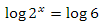
according to the property of logarithms, we can rewrite the equation as follows.
Now we only have to divide both parts by log (2)

But that is not all.X is approximately 2.58. Next, you need to reset the fractional part and build a two to the power of the resulting number. Here is the tessellation factor calculation code for detail levels.
Let's take a look at how you can increase your landscape detail without changing the height map size. The following comes to my mind - change the height value to the value obtained from the gradient noise texture. The coordinates by which we will sample will be N times the major. When sampling, the mirror type of addressing will be used (D3D11_TEXTURE_ADDRESS_MIRROR) (see Figure 14).
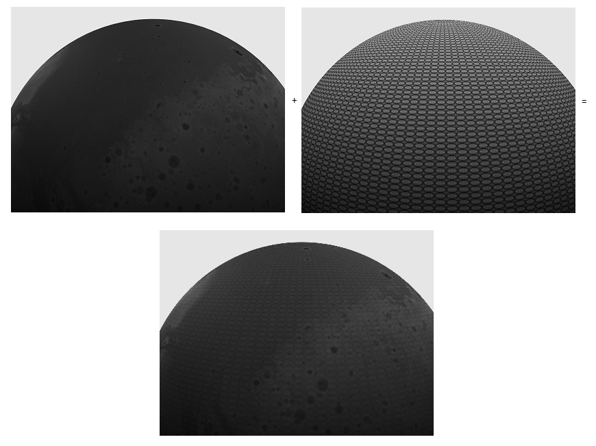
Fig.14 Sphere with height map + sphere with noise map = sphere with final height
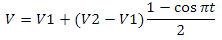
In this case the height will be calculated as follows:
So far, the periodic nature is expressed significantly, but with the addition of lighting and texturing, the situation will change for the better. What is the texture of gradient noise? Roughly speaking, this is a grid of random values. Let's see how to match the size of the lattice to the size of the texture. Suppose we want to create a 256-by-256-pixel noise texture. It's simple, if the dimensions of the lattice coincide with the size of the texture - we get something like white noise on the TV. And what if our lattice has dimensions of, say, 2 by 2? The answer is simple - use interpolation. One of the formulations of linear interpolation is as follows:
This is the fastest, but at the same time the least suitable option. It is better to use cosine-based interpolation:
But we cannot just interpolate between the values along the edges of the diagonal (the lower left and upper right corner of the cell). In our case, the interpolation will need to be applied twice. Let's introduce one of the grid cells. She has four corners - let's call them V1, V2, V3, V4. Also inside this cell there will be its own two-dimensional coordinate system, where the point (0, 0) corresponds to V1 and the point (1, 1) to V3 (see Fig. 15a). In order to get a value with coordinates (0.5, 0.5), we first need to get two values interpolated in X between V1 and V4 and between V2 and V3, and finally interpolate in Y between these values (Fig.15b).
Here is an example:
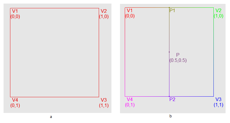
Fig.15 a - Image of a lattice cell with coordinates V1, V2, V3 and V4. b - Sequence of two interpolations on the example of a cell
now let's do the following - for each pixel of the noise texture we take the interpolated value for the 2x2 grid, then add to it the interpolated value for the 4x4 grid multiplied by 0.5, then for the 8x8 grid multiplied by 0.25 and so on. d to a certain limit - this is called the addition of the octaves (Fig. 16). The formula looks like this:

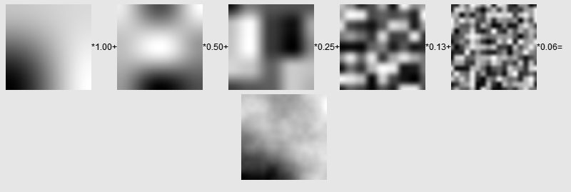
Fig.16 Example of the addition of octaves
Here is an example of the implementation:
Also for V1, V2, V3 and V4 you can get the sum of the value itself and its neighbors as follows:
and use these values in interpolation. Here is the rest of the code:
In the conclusion of the subsection, I want to say that everything I have described up to this point is a slightly different implementation of the Perlin noise.
Deal with the height - now let's see how to deal with the normals. As in the case of the main height map, we need to generate a normal map from the noise text. Then in the shader we simply add the normal from the main card to the normal of the noise texture. I must say that this is not entirely correct, but it gives an acceptable result. Here is an example:
Let's do the optimization. Now the cycle of drawing sectors in pseudocode looks like this
The performance of this approach is extremely small. There are several optimization options - you can build a quad tree for each plane of the cube, so as not to calculate the scalar product for each sector. You can also update the values of V1 and V2 not for each sector, but for the six planes of the cube, which they belong to. I chose the third option - Instancing. Briefly about what it is. Let's say you want to draw a forest. You have a tree model, there is also a set of transformation matrices - tree positions, possible scaling or rotation. You can create one buffer, which will contain the vertices of all trees converted into world space - a good option, the forest does not run on the map. And what if you need to implement transformations - say, swaying trees in the wind.You can do this by copying the data of the model vertices N times into one buffer, adding the tree index to the data of the vertex (from 0 to N). Next, we update the array of transformation matrices and pass it as a variable to the shader. In the shader, we select the desired matrix by the tree index. How can data duplication be avoided? First I want to draw your attention to the fact that these vertices can be collected from several buffers. For when describing a vertex, you need to specify the source index in the InputSlot field of the D3D11_INPUT_ELEMENT_DESC structure. This can be used when implementing morphing facial animation — let's say you have two vertex buffers containing two face states, and you want to interpolate these values linearly. Here's how to describe the top:Next, we update the array of transformation matrices and pass it as a variable to the shader. In the shader, we select the desired matrix by the tree index. How can data duplication be avoided? First I want to draw your attention to the fact that these vertices can be collected from several buffers. For when describing a vertex, you need to specify the source index in the InputSlot field of the D3D11_INPUT_ELEMENT_DESC structure. This can be used when implementing morphing facial animation — let's say you have two vertex buffers containing two face states, and you want to interpolate these values linearly. Here's how to describe the top:Next, we update the array of transformation matrices and pass it as a variable to the shader. In the shader, we select the desired matrix by the tree index. How can data duplication be avoided? First I want to draw your attention to the fact that these vertices can be collected from several buffers. For when describing a vertex, you need to specify the source index in the InputSlot field of the D3D11_INPUT_ELEMENT_DESC structure. This can be used when implementing morphing facial animation — let's say you have two vertex buffers containing two face states, and you want to interpolate these values linearly. Here's how to describe the top:For when describing a vertex, you need to specify the source index in the InputSlot field of the D3D11_INPUT_ELEMENT_DESC structure. This can be used when implementing morphing facial animation — let's say you have two vertex buffers containing two face states, and you want to interpolate these values linearly. Here's how to describe the top:For when describing a vertex, you need to specify the source index in the InputSlot field of the D3D11_INPUT_ELEMENT_DESC structure. This can be used when implementing morphing facial animation — let's say you have two vertex buffers containing two face states, and you want to interpolate these values linearly. Here's how to describe the top:
In the shader, the vertex must be described as follows:
then you just interpolate the values
Why am I doing this? Let's go back to the trees example. The top will be collected from two sources - the first will contain the position in the local space, the texture coordinates and the normal, the second - the transformation matrix in the form of four four-dimensional vectors. The vertex description looks like this:
Note that in the second part, the InputSlotClass field is D3D11_INPUT_PER_INSTANCE_DATA and the InstanceDataStepRate field is one (For a brief description of the InstanceDataStepRate field, see Appendix 1). In this case, the collector will use the entire buffer from a source with type D3D11_INPUT_PER_VERTEX_DATA for each element from a source with type D3D11_INPUT_PER_INSTANCE_DATA. In the shader, these vertices can be described as follows:
By creating a second buffer with the attributes D3D11_USAGE_DYNAMIC and D3D11_CPU_ACCESS_WRITE, we will be able to update it from the CPU. You need to draw this kind of geometry using the calls DrawInstanced () or DrawIndexedInstanced (). There are also calls DrawInstancedIndirect () and DrawIndexedInstancedIndirect () - see Appendix 2 for them.
Let me give an example of setting up buffers and using the DrawIndexedInstanced () function:
Now let's finally get back to our topic. Sector is described by a point on the plane to which it belongs and by two vectors which describe this plane. Therefore, the top will consist of two sources. The first is the coordinates in the grid space, the second is the sector data. The vertex description looks like this:
Please note that I use a three-dimensional vector to store coordinates in the grid space (the z coordinate is not used)
Another important component of optimization is clipping by the pyramid of visibility (Frustum culling). The visibility pyramid is the area of the scene that the camera “sees”. How to build it? First, we recall that a point can be in four coordinate systems — local, world, species, and the projection coordinate system. The transition between them is carried out by means of matrices - world, species and matrix projections, and the transformation must take place sequentially - from the local to the world, from the world to the species and finally from the viewport to the space projection. All these transformations can be combined into one by multiplying these matrices.
We use the perspective projection, which implies the so-called “homogeneous division” - after multiplying the vector (Px, Py, Pz, 1) by the projection matrix, its components should be divided into the W component of this vector. After the transition to the projection space and homogeneous division, the point is in the NDC space. NDC space is a set of three coordinates x, y, z, where x and y belong to [-1, 1], and z - [0,1] (I must say that in OpenGL the parameters are somewhat different).
Now let's get down to solving our problem. In my case, the pyramid is located in the species space. We need six planes that describe it (Fig. 17a). The plane can be described using the normal and the point that belongs to this plane. First, let's get the points - for this we take the following set of coordinates in the NDC space:
Look, at the first four points the value of z is 0 - this means that they belong to the near cut-off plane, at the last four z it is equal to 1 - they belong to the far cut-off plane. Now these points need to be converted into view space. But how?
Remember the example of an astronaut - so here is the same. We need to multiply the points by the inverse projection matrix. True, after that, we still need to divide each of them into its W coordinate. As a result, we will get the necessary coordinates (Fig. 17b). Let's now deal with the normals - they must be directed inside the pyramid, so we need to choose the necessary order of calculation of the vector product.
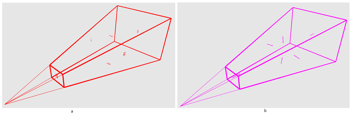
Fig.17 Pyramid of visibility The
pyramid is built - it's time to use it. Those sectors that do not fall inside the pyramid, we do not draw. In order to determine whether a sector is inside the visibility pyramid, we will check the bounding sphere located in the center of this sector. This does not give accurate results, but in this case I do not see anything terrible in the fact that several unnecessary sectors will be drawn. The radius of the sphere is calculated as follows:

where TR is the upper right corner of the sector, BL is the lower left corner. Since all sectors have the same area, it is sufficient to calculate the radius once.
How do we determine if a sphere describing a sector is inside the visibility pyramid? First, we need to determine whether the sphere intersects with the plane and, if not, from which side of it it is located. Let's get a vector on the center of the sphere

where P is a point on the plane and S is the center of the sphere. Now we calculate the scalar product of this vector by the normal to the plane. The orientation can be determined using the mark of the dot product - as mentioned earlier, if it is positive, then the sphere is in front of the plane, if negative, then the sphere is behind. It remains to determine whether the sphere intersects the plane. Let's take two vectors - N (normal vector) and V. Now we construct a vector from N to V - we call it K. Now, we need to find a length N so that it forms a 90 degree angle with K (formally speaking, N and K were orthogonal). Okie doki, look at fig.18a - we know from the properties of a right-angled triangle that we

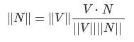
need to find the cosine. Using the previously mentioned scalar product property we

divide both sides by | V | * | N | and get

use this result:
since | V | is just a number, then we can shorten by | V |, and then we get
Since the vector N is normalized, then the last step we simply multiply it by the resulting value, otherwise the vector should be normalized - in this case, the final equation looks like this:
Where D this is our new vector. This process is called "Vector projection" (Fig.18b). But why do we need it? We know that the vector is determined by the length and direction, and does not change from its position - this means that if we place the D so that it pointed to S, its length is equal to the minimum distance from S to the plane (ris.18s)
Figure .18 a Projection of N to V, b Visual display of the length of the projected N as applied to a point, s Visual display
the lengths of the projected N as applied to a sphere centered at S
Since we do not need a projected vector, it suffices to calculate its length. Considering that N is a unit vector, we only need to calculate the scalar product V by N. Putting it all together, we can finally conclude that the sphere intersects the plane if the scalar product of the vector and the center of the sphere and the normal to the plane is greater than zero and less than the radius this sphere.
In order to assert that the sphere is inside the pyramid of visibility, we need to make sure that it either intersects one of the planes, or is in front of each of them. You can put the question to another - if the sphere does not intersect and is behind at least one of the planes - it is definitely out of the pyramid of visibility. So we will do. Note that I translate the center of the sphere into the same space in which the pyramid is located - into the space of the view.
Another problem that we have to solve is cracks at the boundaries of the detail levels (Figure 19).
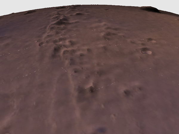
Fig.19 demonstration of landscape cracks.
First of all, we need to identify those sectors that lie on the border of detail levels. At first glance it seems that this is a resource-intensive task - the number of sectors at each level is constantly changing. But if you use the data adjacency, the solution is greatly simplified. What is adjacency data? See, each sector has four neighbors. A set of references to them — be it pointers or indexes — is adjacency data. With their help, we can easily determine which sector lies on the border - it is enough to check which level its neighbors belong to.
Well, let's find the neighbors of each sector. Again, we don’t need to cycle through all sectors. Imagine that we are working with a sector with X and Y coordinates in grid space.
If it does not touch the cube edge, then the coordinates of its neighbors will be as follows:
Neighbor top - (X, Y - 1)
Neighbor bottom - (X, Y + 1)
Neighbor left - (X - 1, Y)
Neighbor right - (X + 1, Y)
If the sector touches the edge, then we place its special container. After processing all six faces, it will contain all the boundary sectors of the cube. It is in this container that we will have to bust. Calculate the edges for each sector in advance:
Next comes the search
The FindSectorEdgeAdjacency () function looks like this
Please note that we update the adjacency data for two sectors - the desired one (Sector) and the found neighbor.
Now, using our adjacency data, we have to find those sector edges that belong to the boundary of detail levels. There is such a plan - before drawing we will find the boundary sectors. Then, for each sector, in addition to the basic
information in the Instance buffer, we write the tessellation coefficient and the four-dimensional vector of tessellation coefficients for the neighboring sectors. The vertex description will now look like this:
After we have divided the sectors by levels of detail, we determine the neighboring tessellation coefficients for each sector:
The function that looks for the next tessellation factor:
If we return zero, then the neighbor on the Side side is of no interest to us. Looking ahead and saying that we need to fix the cracks from the level with a large tessellation coefficient.
Now we go to the shader. Let me remind you that first we need to get the coordinates of the grid, using the coordinates of the tesselator. Then these coordinates are converted to a point on the face of a cube, this point is normalized - and here we have a point on the sphere:
First we need to find out whether the vertex belongs to either the first or last row of the grid, or the first or last column — in this case, the vertex belongs to the edge of the sector. But this is not enough - we need to determine whether the vertex belongs to the level of detail. To do this, we use information about neighboring sectors, or rather their tessellation levels:
Now the main stage - in fact, the elimination of cracks. Look at fig.20. The red line is the vertex of the vertex belonging to the second level of detail. Two blue lines - the faces of the third level of detail. We need to V3 belonged to the red line - that is, lay on the verge of the second level. As both the heights of V1 and V2 are equal for both levels, V3 can be found using linear interpolation between them.
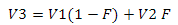

Fig.20 Demonstrating the faces that form a crack in the form of lines
So far we have neither V1 and V2, nor the coefficient F. First we need to find the index of the point V3. Ie, if the grid has a size of 32 by 32 and the tessellation coefficient is four, then this index will be from zero to 128 (32 * 4). We already have coordinates in the grid space p - in the framework of this example, they can be for example (15.5, 16). To obtain the index, multiply one of the coordinates p by the tessellation coefficient. We will also need the beginning of the face and the direction to its end - one of the corners of the sector.
Next, we need to find the indices for V1 and V2. Imagine that you have a number of 3. You need to find the two nearest multiples of two. To do this, you calculate the remainder of dividing three by two - it is equal to one unit. Then you subtract or add this remainder to three and get the desired result. Also with indices, only instead of two we will have a ratio of tessellation coefficients of detail levels. If the third level has a coefficient equal to 16, and the second has 2, then the ratio will be 8. Now, to get the heights, you first need to get the corresponding points on the sphere, normalizing the points on the face. We have already prepared the beginning and direction of the edge - it remains to calculate the length of the vector from V1 to V2. Since the edge length of the cell of the original grid is equal to gridStep.x, then the length we need is equal to gridStep.x / Tri [0] .tessFactor.Then, by points on the sphere, we will get the height, as described earlier.
Well, the last component is the factor F. We get it by dividing the remainder of the division by the ratio of the coefficients (ind) by the ratio of the coefficients (tessRatio)
The final stage is linear interpolation of heights and getting a new vertex.
There may also be a crack in the place where the sectors border on the texture coordinates of the edges equal to 1 or 0. In this case, I take the average value between the heights for the two coordinates:
Let's transfer the processing of sectors to the GPU. We will have two Compute shaders - the first one performs clipping on the visibility pyramid and determines the level of detail, the second one will get the boundary tessellation coefficients to eliminate the cracks. The division into two stages is necessary because, as in the case of the CPU, we cannot correctly determine the neighbors for the sectors until we cut off. Since both shaders will use these levels of detail and work with sectors, I introduced two common structures: Sector and Lod
We will use three main buffers - input (contains the initial information about the sectors), intermediate (it contains data of the sectors obtained as a result of the first stage) and final (Will be transferred to the drawing). The input buffer data will not change, so in the Usage field of the D3D11_BUFFER_DESC structure, it is reasonable to use the value of D3D11_USAGE_IMMUTABLE We simply write data from all sectors with the only difference that we will use sector indices instead of pointers to these adjacency data. For the index of the level of detail and the boundary coefficients of tessellation set zero values:
Now a couple of words about the intermediate buffer. It will play two roles - output for the first shader and input for the second, so we will indicate in the BindFlags field the value D3D11_BIND_UNORDERED_ACCESS | D3D11_BIND_SHADER_RESOURCE. We will also create for it two mappings - UnorderedAccessView, which will allow the shader to write to it the result of the work and the ShaderResourceView, with which we will use the buffer as input. Its size will be the same as the previously created input buffer.
Next, I will give the main function of the first shader:
After calculating the dot product, we check if the sector is in a potentially visible area. Next, we clarify the fact of its visibility using the IsVisible () call, which is identical to the Frustum :: TestSphere () call shown earlier. The function depends on the worldView, sphereRadius, frustumPlanesPosV and frustumPlanesNormalsV variables, the values for which need to be passed to the shader in advance. Next, we determine the level of detail. Please note that we specify the level index from a unit - this is necessary in order to discard those sectors whose level of detail is zero at the second stage.
Now we need to prepare buffers for the second stage. We want to use the buffer as output for the Compute shader and input for the tesselitator - for this we need to specify the value D3D11_BIND_UNORDERED_ACCESS | in the BindFlags field. D3D11_BIND_VERTEX_BUFFER. We will have to work with the buffer data directly, so we specify the value D3D11_RESOURCE_MISC_BUFFER_ALLOW_RAW_VIEWS in the MiscFlags field. To display this buffer, we will use the value DXGI_FORMAT_R32_TYPELESS in the Flags field, and in the NumElements field we specify the entire buffer, in the Flags field, in the Flags field, in the Flags field, in the Flags field, in the Flags field, in the Flags field, in the Flags field, in the Flags field, in the Flags field, we specify the entire buffer, in the Flags field, and in the Flags field, we will use the entire buffer, in the Flags field, we will use the entire buffer, in the Flags field, we will use the buffer in the Flags field;
We also need a counter. With it, we will address the memory in the shader and use its final value in the instanceCount argument of the drawIndexedInstanced () call. The counter I implemented in the form of a buffer of 16 bytes. Also, when creating the display in the Flags field of the D3D11_BUFFER_UAV field, I used the value D3D11_BUFFER_UAV_FLAG_COUNTER
It is time to bring the code of the second shader
The function code GetNeibTessFactor () is almost identical to its CPU counterpart. The only difference is that we use neighbor indices and not pointers to them. The outputData buffer is of type RWByteAddressBuffer, so we use the Store method (in uint address, in uint value) to work with it. The value of the variable dataSize is equal to the size of the vertex data with the class D3D11_INPUT_PER_INSTANCE_DATA, the description of the vertex can be viewed in section 10. In general, this is traditional for C / C ++ working with pointers. After executing the two shaders, we can use outputData as an InstanceBuffer. The rendering process looks like this.
For more information about the DrawIndexedInstancedIndirect () and CopyStructureCount () methods, see Appendix 2.
Surely you know how to model a simple FPS (First Person Shooter) camera model. I act according to this scenario:
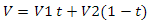
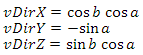
In our case, the situation is somewhat complicated - firstly we must move relative to the center of the planet, secondly, when constructing the basis, instead of the vector (0, 1, 0), we must use the normal of the sphere at the point we are in now. To achieve the desired results, I will use two bases. According to the first, the position will change, the second will describe the orientation of the camera. The bases are interdependent, but I first calculate the basis of the position, so I'll start with it. Suppose we have an initial position basis (pDir, pUp, pRight) and a direction vector vDir, in which we want to move some distance. First of all, we need to calculate the projections of vDir on pDir and pRight. Having added them, we will receive the updated direction vector (Fig. 21).
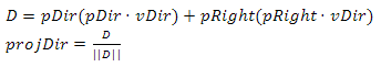

Fig.21 The visual process of getting projDir
Next we move along this vector

where P is the camera position, mF and mS are the coefficients, which means how much we need to move forward or sideways.
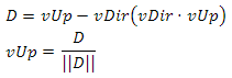
We cannot use PN as a new camera position, because PN does not belong to a sphere. Instead, we find the normal of the sphere at the point PN, and this normal will be the new value of the vector up. Now we can form an updated basis
where spherePos is the center of the sphere.
We need to make sure that each of its vectors is orthogonal to the other two. According to the property of the vector product, nRight satisfies this condition. It remains to achieve the same for nUp and nDir. To do this, project nDir onto nUp and subtract the resulting vector from nDir (Fig.22) Fig.22
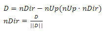

Orthogonalizing nDir with respect to nUp
We could do the same with nUp, but then it would change its direction, which in our case is unacceptable. Now we normalize nDir and obtain an updated orthonormal direction basis.
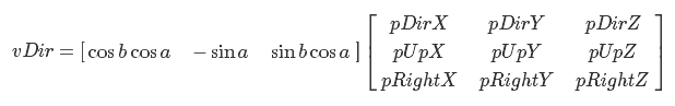
The second key step is to build the basis of orientation. The main difficulty is getting the direction vector. the most suitable solution is to convert a point with a polar angle a, an azimuth angle b and a distance from the origin of coordinates equal to one from spherical coordinates to Cartesian. Only if we make such a transition for a point with a polar angle equal to zero, then we get a vector looking up. This does not quite suit us, since we will increment the angles and assume that such a vector will look ahead. A banal angle shift of 90 degrees will solve the problem, but it will be more elegant to use the angle shift rule, which says that
we will do so. As a result, we have the following:
where a is the polar angle, b is the azimuth angle.
This result does not quite suit us - we need to build a direction vector relative to the basis of the position. Let's rewrite the equation for vDir:

Everything, like astronauts - in this direction so much, so much so. Now it should be obvious that if we replace the vectors of the standard basis with pDir, pUp and pRight, then we get the direction we need. So you

can imagine the same thing in the form of matrix multiplication. The
vector vUp will initially be equal to pUp. Having calculated the vector product vUp and vDir, we get vRight.

Now we will make it so that vUp is orthogonal with respect to the other vectors of the basis. The principle is the same as when working with nDir.
The bases were sorted out - it remains to calculate the camera position. This is done like this.

where spherePos is the center of the sphere, sphereRadius is the radius of the sphere and height is the height above the surface of the sphere. I will give the code of operation of the camera described:
Please note that we reset angles.x after we have updated the basis of the position. This is critically important. Let's imagine that we simultaneously change the angle of view and move around the sphere. First, we project the direction vector onto pDir and pRight, get the offset (newPos) and, based on it, update the position basis. The second condition will also work, and we will begin to update the orientation basis. But since pDir and pRight have already been changed depending on vDir, then without resetting the azimuth angle (angles.x), the rotation will be more “steep”
I thank the reader for showing interest in the article. I hope that the information contained therein was accessible, interesting and useful. Suggestions and comments can be sent to me by mail alexwin32@mail.ru or leave as comments.
I wish you success!
Fig.1 elevation map + plane = landscape
Why does this work? If we imagine that the player is on the surface of the sphere, and the radius of this sphere is extremely large relative to the size of the player, then the curvature of the surface can be neglected and the plane can be used. But what if we do not neglect the fact that we are on a sphere? I want to share my experience in building such landscapes with the reader in this article.
1. Sector
Obviously, it is not reasonable to build a landscape at once for the whole sphere - most of it will not be visible. Therefore, we need to create a certain minimum area of space - a certain primitive, of which the relief of the visible part of the sphere will consist. I will call it a sector. How do we get it? So look at fig.2a. The green box is our sector. Next, we construct six grids, each of which is a cube face (Fig. 2b). Now let's normalize the coordinates of the primitives that form the grids (Fig. 2c).
')
Pic2
As a result, we got a cube projected onto a sphere, where the sector is the area on one of its faces. Why does this work? Consider an arbitrary point on the grid as a vector from the origin. What is vector normalization? This is a transformation of a given vector into a vector in the same direction, but with a unit length. The process is as follows: first we find the length of the vector in the Euclidean metric according to the Pythagorean theorem
Then we divide each of the vector components into this value.
Now we ask ourselves what is a sphere? A sphere is a set of points equidistant from a given point. The parametric sphere equation looks like this.
where x0, y0, z0 are the coordinates of the center of the sphere, and R is its radius. In our case, the center of the sphere is the origin, and the radius is one. Substitute the known values and take the root of the two parts of the equation. It turns out the following
Literally, the last transformation tells us the following: “In order to belong to a sphere, the vector length must be equal to one”. This we have achieved normalization.
What if the sphere has an arbitrary center and radius? Find the point that belongs to her by using the following equation
where pS is a point on the sphere, C is the center of the sphere, pNorm is the previously normalized vector and R is the radius of the sphere. In simple words, the following happens here: “we move from the center of the sphere towards the point on the grid at a distance R”. Since each vector has a unit length, in the end, all points are equidistant from the center of the sphere at a distance of its radius, which makes the equation of the sphere true.
2. Management
We need to get a group of sectors that are potentially visible from the viewpoint. But how to do that? Suppose we have a sphere with center at some point. We also have a sector that is located on a sphere and a point P located in the space near the sphere. Now we construct two vectors - one directed from the center of the sphere to the center of the sector, the other from the center of the sphere to the point of view. Look at Figure 3 - a sector can only be seen if the absolute value of the angle between these vectors is less than 90 degrees.
Fig.3 a - angle less than 90 - the sector is potentially visible. b - angle greater than 90 - sector is not visible
How to get this angle? To do this, use the scalar product of vectors. For the three-dimensional case, it is calculated as:
Scalar product has a distribution property:
Earlier, we defined the vector length equation - now we can say that the length of the vector is equal to the root of the scalar product of this vector itself. Or vice versa - the scalar product of the vector itself is equal to the square of its length.
Now let's turn to the law of cosines. One of his two formulations looks like this (Fig. 4):
Fig.4 cosine law
If we take the lengths of our vectors as a and b, then the angle alfa is what we are looking for. But how do we get value with? See: if we take a from b, then we get a vector directed from a to b, and since the vector is characterized only by direction and length, then we can graphically arrange its beginning at the end of vector a. From this, we can say that c is equal to the length of the vector b - a. So we did
Express the squares of lengths as scalar products
open brackets using the distribution property
a little shorten
and finally, by dividing both equations of the equation by minus two, we get
This is another property of the scalar product. In our case, we need to normalize the vectors so that their lengths are equal to one. We don’t need to calculate the angle - the cosine value is enough. If it is less than zero, then we can safely say that we are not interested in this sector.
3. Grid
It's time to think about how to draw primitives. As I said earlier, the sector is the main component in our scheme, so for each potentially visible sector we will draw a grid, the primitives of which will form the landscape. Each of its cells can be displayed using two triangles. Due to the fact that each cell has adjacent faces, the values of most triangle vertices are repeated for two or more cells. Not to duplicate the data in the vertex buffer, fill the index buffer. If indices are used, then with their help the graphic pipeline determines which primitive in the vertex buffer to process. (pic.5) The topology I chose is a triangle list (D3D11_PRIMITIVE_TOPOLOGY_TRIANGLELIST)
Fig.5 Visual display of indexes and primitives
Creating a separate vertex buffer for each sector is too expensive. It is much more efficient to use one buffer with coordinates in the grid space, that is, x is a column and y is a row. But how to get a point on the sphere from them? A sector is a square area with a beginning at a certain point S. All sectors have the same length of the face - let's call it SLen. The grid covers the entire area of the sector and also has the same number of rows and columns, so we can build the following equation to find the length of the cell face.
where CLen is the length of the cell face, MSize is the number of rows or columns of the grid. We divide both parts by MSize and get CLen
We go further. The space of the face of the cube to which the sector belongs can be expressed as a linear combination of two vectors of unit length — we call them V1 and V2. We have the following equation (see fig. 6)
Fig.6 A visual representation of the formation of a point on the grid
to get a point on a sphere, we use the equation derived earlier
4. Height
All that we have achieved by this moment is not very similar to the landscape. It's time to add what will make it so - the difference in height. Let's imagine that we have a sphere of unit radius with center at the origin of coordinates, as well as a set of points {P0, P1, P2 ... PN}, which are located on this sphere. Each of these points can be represented as a unit vector from the origin. Now imagine that we have a set of values, each of which is the length of a particular vector (Fig. 7).
I will store these values in a two-dimensional texture. We need to find the relationship between the coordinates of the pixel texture and the vector-point on the sphere. Let's get started
In addition to Cartesian, a point on a sphere can also be described using a spherical coordinate system. In this case, its coordinates will consist of three elements: the azimuth angle, the polar angle, and the value of the shortest distance from the origin to the point. The azimuth angle is the angle between the X axis and the projection of the ray from the origin to a point on the XZ plane. It can take values from zero to 360 degrees. Polar angle - the angle between the Y axis and the ray from the origin to the point. It can also be called zenith or normal. Accepts values from zero to 180 degrees. (see figure 8)
Fig.8 Spherical coordinates
To go from a Cartesian system to a spherical, I use the following equations (I believe that the Y axis is pointing up):
where d is the distance to the point, a is the polar angle, b is the azimuth angle. The parameter d can also be described as “the length of the vector from the origin to the point” (as can be seen from the equation). If we use normalized coordinates, we can avoid division when finding the polar angle. Actually, why do we need these corners? Dividing each of them into its maximum range, we obtain coefficients from zero to one and with their help we will select the texture from the shader. When obtaining the coefficient for the polar angle, it is necessary to take into account the quarter in which the angle is located. "But the value of the expression z / x is not defined when x is equal to zero" - you say. I will say more: when z equals zero, the angle will be zero regardless of the value of x.
Let's add some special cases for these values. We have normalized coordinates (normal) - we add several conditions: if the X value of the normal is zero and the Z value is greater than zero, then the coefficient is 0.25, if X is zero and Z is less than zero, then it will be 0.75. If the value of Z is zero and X is less than zero, then in this case the coefficient will be equal to 0.5. All this is easy to check on the circumference. But what to do if Z is zero and X is greater than zero - in this case, both 0 and 1 will be correct? Imagine that we chose 1 — well, let's take a sector with a minimum azimuth angle of 0 and a maximum angle of 90 degrees. Now consider the first three vertices in the first row of the grid that displays this sector. For the first vertex, we met the condition and set the textural coordinate of X to 1. It is obvious that for the next two vertices this condition will not be fulfilled - the angles for them are in the first quarter and as a result we get something like this - (1.0, 0.05, 0.1). But for a sector with angles from 270 to 360 for the last three vertices in the same line, everything will be correct - the condition for the last vertex will work, and we will get a set (0.9, 0.95, 1.0). If we choose zero as the result, we get sets (0.0, 0.05, 0.1) and (0.9, 0.95, 0.0) - in any case, this will lead to quite noticeable distortions of the surface. So let's apply the following. Take the center of the sector, then normalize its center, thereby moving it onto the sphere. Now we calculate the scalar product of the normalized center by the vector (0, 0, 1). Formally speaking, this vector is normal to the XY plane, and by calculating its scalar product with the normalized vector of the center of the sector, we can understand which side of the plane the center is from. If it is less than zero, then the sector is behind the plane and we need the value 1. If the scalar product is greater than zero, then the sector is in front of the plane and therefore the boundary value is 0. (see Fig.9)
Fig.9 The problem of choosing between 0 and 1 for texture coordinates
Here is the code for obtaining texture coordinates from spherical. Please note that because of the error in the calculations, we cannot check the values of the normal for equality to zero, instead we must compare their absolute values with a certain threshold value (for example, 0.001)
//norm - , //offset - , norm //zeroTreshold - (0.001) float2 GetTexCoords(float3 norm, float3 offset) { float tX = 0.0f, tY = 0.0f; bool normXIsZero = abs(norm.x) < zeroTreshold; bool normZIsZero = abs(norm.z) < zeroTreshold; if(normXIsZero || normZIsZero){ if(normXIsZero && norm.z > 0.0f) tX = 0.25f; else if(norm.x < 0.0f && normZIsZero) tX = 0.5f; else if(normXIsZero && norm.z < 0.0f) tX = 0.75f; else if(norm.x > 0.0f && normZIsZero){ if(dot(float3(0.0f, 0.0f, 1.0f), offset) < 0.0f) tX = 1.0f; else tX = 0.0f; } }else{ tX = atan(norm.z / norm.x); if(norm.x < 0.0f && norm.z > 0.0f) tX += 3.141592; else if(norm.x < 0.0f && norm.z < 0.0f) tX += 3.141592; else if(norm.x > 0.0f && norm.z < 0.0f) tX = 3.141592 * 2.0f + tX; tX = tX / (3.141592 * 2.0f); } tY = acos(norm.y) / 3.141592; return float2(tX, tY); } I will give an intermediate version of the vertex shader
//startPos - //vec1, vec2 - //gridStep - //sideSize - //GetTexCoords() - VOut ProcessVertex(VIn input) { float3 planePos = startPos + vec1 * input.netPos.x * gridStep.x + vec2 * input.netPos.y * gridStep.y; float3 sphPos = normalize(planePos); float3 normOffset = normalize(startPos + (vec1 + vec2) * sideSize * 0.5f); float2 tc = GetTexCoords(sphPos, normOffset); float height = mainHeightTex.SampleLevel(mainHeightTexSampler, tc, 0).x; posL = sphPos * (sphereRadius + height); VOut output; output.posH = mul(float4(posL, 1.0f), worldViewProj); output.texCoords = tc; return output; } 5. Lighting
In order to realize the dependence of the landscape color on lighting, we will use the following equation:
Where I is the color of the point, Ld is the color of the light source, Kd is the color of the material of the illuminated surface, a is the angle between the vector of the source and the normal to the illuminated surface. This is a special case of the Lambert cosine law. Let's see what is here and why. By multiplying Ld by Kd is meant componentwise color multiplication, that is (Ld.r * Kd.r, Ld.g * Kd.g, Ld.b * Kd.b). It may be easier to understand the meaning if we imagine the following situation: suppose we want to illuminate an object with a green light source, so we expect the color of the object to be in gradations of green. The result (0 * Kd.r, 1 * Kd.g, 0 * Kd.b) gives (0, Kd.g, 0) - exactly what we need. We go further. As stated earlier, the cosine of the angle between normalized vectors is their scalar product. Let's look at its maximum and minimum value from our point of view. If the cosine of the angle between the vectors is 1, then this angle is 0 - therefore, both vectors are collinear (lie on the same line).
The same is true for the cosine value of -1, only in this case the vectors point in opposite directions. It turns out, the closer the normal vector and the vector to the light source to the state of collinearity - the higher the luminance factor of the surface to which the normal belongs. It is also assumed that the surface cannot be illuminated if its normal points in the direction opposite to the direction to the source — that is why I use only positive cosine values.
I use a parallel source, so its position can be neglected. The only thing that needs to be taken into account is that we use a vector to the light source. That is, if the direction of the rays is (1.0, -1.0, 0) - we need to use the vector (-1.0, 1.0, 0). The only thing that is difficult for us is the normal vector. It is easy to calculate the normal to the plane - we need to produce the vector product of two vectors that describe it. It is important to remember that the vector product is anticommutative - you need to take into account the order of the factors. In our case, we can obtain the normal to the triangle, knowing the coordinates of its vertices in the space of the grid, as follows (Note that I do not take into account the boundary cases for px and py)
float3 p1 = GetPosOnSphere(p); float3 p2 = GetPosOnSphere(float2(px + 1, py)); float3 p3 = GetPosOnSphere(float2(px, py + 1)); float3 v1 = p2 - p1; float3 v2 = p3 - p1; float3 n = normalzie(cross(v1, v2)); But that is not all. Most vertices of the grid belong immediately to four planes. To get an acceptable result, you need to calculate the average normal as follows:
Na = normalize(n0 + n1 + n2 + n3) Implementing this method on a GPU is quite expensive - we need two steps to calculate the normals and average them. In addition, the efficiency leaves much to be desired. Based on this, I chose another way - to use the normal map. (Fig.10)
Pic.10 Normal map
The principle of working with it is the same as with the height map - we transform the spherical coordinates of the grid vertex into textural coordinates and make a selection. Only we will not be able to use this data directly - after all, we work with the sphere, and the vertex has its own normal, which must be taken into account. Therefore, we will use the data of the normal map as the coordinates of the TBN basis. What is a basis? Here is an example. Imagine that you are an astronaut and are sitting on a beacon somewhere in space. You receive a message from the MCC: “You need to move from the beacon 1 meter to the left, 2 meters up and 3 meters ahead.” How can this be mathematically expressed? (1, 0, 0) * 1 + (0, 1, 0) * 2 + (0, 0, 1) * 3 = (1,2,3). In matrix form, this equation can be expressed as:
Now imagine that you are also sitting on the beacon, only now they write to you from the MCC: “we sent you direction vectors there - you have to move 1 meter along the first vector, 2 meters along the second and 3 along the third”. The equation for the new coordinates will be:
component entry is as follows:
Or in matrix form:
so, the matrix with the vectors V1, V2 and V3 is the basis, and the vector (1,2,3) is the coordinates in the space of this basis.
Imagine now that you have a set of vectors (basis M) and you know where you are relative to the beacon (point P). You need to know your coordinates in the space of this base - how much you need to move along these vectors to be in the same place. Imagine the required coordinates (X)
If P, M and X were numbers, we would simply divide both sides of the equation into M, but alas ... Let's go the other way - according to the property of the inverse matrix
where I is the identity matrix. In our case, it looks like this.
What does this give us? Try multiplying this matrix by X and you will get
It is also necessary to clarify that the multiplication of matrices has the property of associativity
We can legitimately consider the vector as a 3 on 1 matrix.
Considering the above, we can conclude that in order to get X in the right side of the equation, we need to multiply both sides in the correct order by the inverse M matrix
We will need this result in the future.
Now back to our problem. I will use an orthonormal basis, which means that V1, V2 and V3 are orthogonal with respect to each other (form an angle of 90 degrees) and have a unit length. The tangent vector will act as V1, V2 - bitangent vector, V3 - normal. In the traditional DirectX transposed form, the matrix looks like this:
where T is the tangent vector, B is the bitangent vector and N is the normal. Let's find them. With the normal, the easiest thing to do is essentially the normalized coordinates of a point. Bitangent vector is equal to the vector product of the normal and tangent vector. The hardest thing to do is with the tangent vector. It is equal to the direction of the tangent to the circle at the point. Let's break this down. First we find the coordinates of a point on the unit circle in the XZ plane for some angle a
The direction of the tangent to the circle at this point can be found in two ways. The vector to the point on the circle and the tangent vector are orthogonal — therefore, since the sin and cos functions are periodic, we can simply add pi / 2 to the angle a and obtain the desired direction. According to the bias property on pi / 2:
we have the following vector:
We can also use differentiation - see Appendix 3 for more details. Thus, in Figure 11 you can see a sphere, for each vertex of which a basis is built. Blue vectors are normals, red tangent vectors, green bitangent vectors.
Fig.11 Sphere with TBN bases at each vertex. Red - tangent vectors, green - bitangent vectors, blue vectors - normals
With the base figured out - now let's get the normal map. To do this, use the Sobel filter. The Sobel filter computes the gradient of the brightness of the image at each point (roughly speaking, the vector of brightness change). The principle of the filter is that you need to apply a certain matrix of values, which is called the "Core", to each pixel and its neighbors within the dimension of this matrix. Suppose that we process pixel P with the K kernel. If it is not on the border of the image, then it has eight neighbors — the left top, top, right top, and so on. We call them tl, t, tb, l, r, bl, b, br. So, the application of the K kernel to this pixel is as follows:
Pn = tl * K (0, 0) + t * K (0,1) + tb * K (0,2) +
& nbsp & nbsp & nbsp & nbsp & nbsp & nbsp & nbsp & nbsp & nbsp & nbspl * K (1, 0) + P * K (1,1) + r * K (1,2) +
& nbsp & nbsp & nbsp & nbsp & nbsp & nbsp & nbsp & nbsp & nbsp & nbspbl * K (2, 0) + b * K (2.1) + br * K (2.2)
This process is called "convolution." The Sobel filter uses two cores to compute the gradient vertically and horizontally. Denote them as Kx and K:
The basis is - you can begin to implement. First we need to calculate the pixel brightness. I use the conversion from the RGB color model to the YUV model for the PAL system:
But since our image is originally in grayscale, this stage can be skipped. Now we need to “collapse” the original image with the Kx and Ky cores. So we get the X and Y components of the gradient. The value of the normal of this vector may also be very useful - we will not use it, but images containing normalized values of the normal of the gradient have several useful applications. By normalization, I mean the following equation
where V is the value that we normalize, Vmin and Vmax are the range of these values. In our case, the minimum and maximum values are tracked during the generation process. Here is an example of the implementation of the Sobel filter:
float SobelFilter::GetGrayscaleData(const Point2 &Coords) { Point2 coords; coords.x = Math::Saturate(Coords.x, RangeI(0, image.size.width - 1)); coords.y = Math::Saturate(Coords.y, RangeI(0, image.size.height - 1)); int32_t offset = (coords.y * image.size.width + coords.x) * image.pixelSize; const uint8_t *pixel = &image.pixels[offset]; return (image.pixelFormat == PXL_FMT_R8) ? pixel[0] : (0.30f * pixel[0] + //R 0.59f * pixel[1] + //G 0.11f * pixel[2]); //B } void SobelFilter::Process() { RangeF dirXVr, dirYVr, magNormVr; for(int32_t y = 0; y < image.size.height; y++) for(int32_t x = 0; x < image.size.width; x++){ float tl = GetGrayscaleData({x - 1, y - 1}); float t = GetGrayscaleData({x , y - 1}); float tr = GetGrayscaleData({x + 1, y - 1}); float l = GetGrayscaleData({x - 1, y }); float r = GetGrayscaleData({x + 1, y }); float bl = GetGrayscaleData({x - 1, y + 1}); float b = GetGrayscaleData({x , y + 1}); float br = GetGrayscaleData({x + 1, y + 1}); float dirX = -1.0f * tl + 0.0f + 1.0f * tr + -2.0f * l + 0.0f + 2.0f * r + -1.0f * bl + 0.0f + 1.0f * br; float dirY = -1.0f * tl + -2.0f * t + -1.0f * tr + 0.0f + 0.0f + 0.0f + 1.0f * bl + 2.0f * b + 1.0f * br; float magNorm = sqrtf(dirX * dirX + dirY * dirY); int32_t ind = y * image.size.width + x; dirXData[ind] = dirX; dirYData[ind] = dirY; magNData[ind] = magNorm; dirXVr.Update(dirX); dirYVr.Update(dirY); magNormVr.Update(magNorm); } if(normaliseDirections){ for(float &dirX : dirXData) dirX = (dirX - dirXVr.minVal) / (dirXVr.maxVal - dirXVr.minVal); for(float &dirY : dirYData) dirY = (dirY - dirYVr.minVal) / (dirYVr.maxVal - dirYVr.minVal); } for(float &magNorm : magNData) magNorm = (magNorm - magNormVr.minVal) / (magNormVr.maxVal - magNormVr.minVal); } I must say that the Sobel filter has the property of linear separability, so this method can be optimized.
The difficult part is over - it remains to record the X and Y coordinates of the gradient direction in the R and G channels of the pixels of the normal map. For the Z coordinates, I use a unit. I also use a three-dimensional vector of coefficients to adjust these values. The following is an example of generating a normal map with comments:
//ImageProcessing::ImageData Image - . ImageProcessing::SobelFilter sobelFilter; sobelFilter.Init(Image); sobelFilter.NormaliseDirections() = false; sobelFilter.Process(); const auto &resX =sobelFilter.GetFilteredData(ImageProcessing::SobelFilter::SOBEL_DIR_X); const auto &resY =sobelFilter.GetFilteredData(ImageProcessing::SobelFilter::SOBEL_DIR_Y); ImageProcessing::ImageData destImage = {DXGI_FORMAT_R8G8B8A8_UNORM, Image.size}; size_t dstImageSize = Image.size.width * Image.size.height * destImage.pixelSize; std::vector<uint8_t> dstImgPixels(dstImageSize); for(int32_t d = 0 ; d < resX.size(); d++){ // . (0.03, 0.03, 1.0) Vector3 norm = Vector3::Normalize({resX[d] * NormalScalling.x, resY[d] * NormalScalling.y, 1.0f * NormalScalling.z}); Point2 coords(d % Image.size.width, d / Image.size.width); int32_t offset = (coords.y * Image.size.width + coords.x) * destImage.pixelSize; uint8_t *pixel = &dstImgPixels[offset]; // [-1.0, 1.0] [0.0, 1.0] [0, 256] pixel[0] = (0.5f + norm.x * 0.5f) * 255.999f; pixel[1] = (0.5f + norm.y * 0.5f) * 255.999f; pixel[2] = (0.5f + norm.z * 0.5f) * 255.999f; } destImage.pixels = &dstImgPixels[0]; SaveImage(destImage, OutFilePath); Now I will give an example of using the normal map in the shader:
//texCoords - , .4 //normalL - //lightDir - //Ld - //Kd - float4 normColor = mainNormalTex.SampleLevel(mainNormalTexSampler, texCoords, 0); // [0.0, 1.0] [-1.0, 1.0] float3 normalT = normalize(2.0f * mainNormColor.rgb - 1.0f); // [0.0, 1.0] [0.0, Pi*2.0] float ang = texCoords.x * 3.141592f * 2.0f; float3 tangent; tangent.x = -sin(ang); tangent.y = 0.0f; tangent.z = cos(ang); float3 bitangent = normalize(cross(normalL, tangent)); float3x3 tbn = float3x3(tangent, bitangent, normalL); float3 resNormal = mul(normalT, tbn); float diff = saturate(dot(resNormal, lightDir.xyz)); float4 resColor = Ld * Kd * diff; 6. Level Of Detail
Well, now our landscape is lit! You can fly to the moon - we zaguraem height map, set the color of the material, load the sectors, set the grid size to {16, 16} and ... Yes, something is not enough - put it on {256, 256} - oh, something slows down , and why high detail on distant sectors? Moreover, the closer the observer to the planet, the smaller sectors he can see. Yes ... we still have a lot of work to do! Let's first figure out how to cut off the extra sectors. The determining value here will be the height of the observer from the surface of the planet - the higher it is, the more sectors it can see (Figure 12)
Fig.12. Dependence of the height of the observer on the number of sectors being processed.
We find the height as follows: we construct the vector from the observer’s position to the center of the sphere, calculate its length and subtract the value of the radius of the sphere from it. Earlier, I said that if the scalar product of the vector on the observer and the vector on the center of the sector is less than zero, then this sector does not interest us - now instead of zero we will use a value linearly dependent on height. First let's define the variables - so we will have the minimum and maximum values of the scalar product and the minimum and maximum values of the height. Construct the following system of equations
Now we express A in the second equation
substitute A from the second equation into the first
express B from the first equation
we substitute B from the first equation into the second
Now we will substitute variables in function
and get
Where Hmin and Hmax are the minimum and maximum heights, Dmin and Dmax are the minimum and maximum values of the scalar product. This problem can be solved differently - see Appendix 4.
Now you need to understand the levels of detail. Each of them will determine the region of the value of the scalar product. In pseudocode, the process of determining whether a sector belongs to a certain level looks like this:
, We need to calculate the range for each level. First, we construct a system of two equations
deciding it, we get
Using these coefficients, we define the function
where Rmax is the domain of the scalar product (D (H) - Dmin), Rmin is the minimum domain defined by the level. I use the value of 0.01. Now we need to subtract the result from Dmax
C using this function, we obtain areas for all levels. Here is an example:
const float dotArea = dotRange.maxVal - dotRange.minVal; const float Rmax = dotArea, Rmin = 0.01f; float lodsCnt = lods.size(); float A = Rmax; float B = powf(Rmin / Rmax, 1.0f / (lodsCnt - 1.0f)); for(size_t g = 0; g < lods.size(); g++){ lods[g].dotRange.minVal = dotRange.maxVal - A * powf(B, g); lods[g].dotRange.maxVal = dotRange.maxVal - A * powf(B, g + 1); } lods[lods.size() - 1].dotRange.maxVal = 1.0f; Now we can determine to which level of detail the sector belongs (Fig. 13).
Fig.13 Color differentiation of sectors according to levels of detail
Next you need to deal with the size of the grid. It will be very expensive to store your grid for each level - it is much more efficient to change the detail of one grid on the fly using tessellation. To do this, in addition to the above-vertex and pixel ones, we also need to implement hull and domain shaders. In the Hull shader, the main task is to prepare control points. It consists of two parts - the main function and the function that calculates the parameters of the control point. Be sure to specify values for the following attributes:
domainHere is an example of a hull shader for splitting triangles:
partitioning
outputtopology
outputcontrolpoints
patchconstantfunc
struct PatchData { float edges[3] : SV_TessFactor; float inside : SV_InsideTessFactor; }; PatchData GetPatchData(InputPatch<VIn, 3> Patch, uint PatchId : SV_PrimitiveID) { PatchData output; flloat tessFactor = 2.0f; output.edges[0] = tessFactor; output.edges[1] = tessFactor; output.edges[2] = tessFactor; output.inside = tessFactor; return output; } [domain("tri")] [partitioning("integer")] [outputtopology("triangle_cw")] [outputcontrolpoints(3)] [patchconstantfunc("GetPatchData")] VIn ProcessHull(InputPatch<VIn, 3> Patch, uint PointId : SV_OutputControlPointID, uint PatchId : SV_PrimitiveID) { return Patch[PointId]; } See, the main work is done in GetPatchData (). Her task is to establish the tessellation factor. We will talk about it later, now we will pass to the Domain shader. It receives control points from the Hull shader and coordinates from the tesselator. The new value of the position or texture coordinates in the case of splitting triangles must be calculated by the following formula
N = C1 * Fx + C2 * Fy + C3 * Fz
where C1, C2 and C3 are the values of the control points, F are the tesselator coordinates. Also in the Domain shader, you need to set the domain attribute, the value of which corresponds to that specified in the Hull shader. Here is an example of the Domain shader:
cbuffer buff0 : register(b0) { matrix worldViewProj; } struct PatchData { float edges[3] : SV_TessFactor; float inside : SV_InsideTessFactor; }; [domain("quad")] PIn ProcessDomain(PatchData Patch, float3 Coord : SV_DomainLocation, const OutputPatch<VIn, 3> Tri) { float3 posL = Tri[0].posL * Coord.x + Tri[1].posL * Coord.y + Tri[2].posL * Coord.z; float2 texCoords = Tri[0].texCoords * Coord.x + Tri[1].texCoords * Coord.y + Tri[2].texCoords * Coord.z; PIn output; output.posH = mul(float4(posL, 1.0f), worldViewProj); output.normalW = Tri[0].normalW; output.texCoords = texCoords; return output; } The role of the vertex shader in this case is minimized - for me it simply “drives” the data to the next stage.
Now you need to implement something similar. Our primary task is to calculate the tessellation factor, or more precisely, to build its dependence on the height of the observer. Again, build a system of equations
deciding it in the same way as before, we get
where Tmin and Tmax are the minimum and maximum tessellation coefficients, Hmin and Hmax are the minimum and maximum values of the observer height. My minimum tessellation coefficient is one. maximum is set separately for each level
(for example 1, 2, 4, 16).
In the future we will need to growth factor was limited to the nearest degree of two.that is, for values from two to three we set the value to two, for values from 4 to 7 we set 4, with values from 8 to 15, the factor will be equal to 8, etc. Let's solve this problem for factor 6. First,
let's solve the following equation. Let's take the decimal logarithm of the two parts of the equation
according to the property of logarithms, we can rewrite the equation as follows.
Now we only have to divide both parts by log (2)
But that is not all.X is approximately 2.58. Next, you need to reset the fractional part and build a two to the power of the resulting number. Here is the tessellation factor calculation code for detail levels.
float h = camera->GetHeight(); const RangeF &hR = heightRange; for(LodsStorage::Lod &lod : lods){ //derived from system //A + B * Hmax = Lmin //A + B * Hmin = Lmax //and getting A then substitution B in second equality float mTf = (float)lod.GetMaxTessFactor(); float tessFactor = 1.0f + (mTf - 1.0f) * ((h - hR.maxVal) / (hR.minVal - hR.maxVal)); tessFactor = Math::Saturate(tessFactor, RangeF(1.0f, mTf)); float nearPowOfTwo = pow(2.0f, floor(log(tessFactor) / log(2))); lod.SetTessFactor(nearPowOfTwo); } 7. Noise
Let's take a look at how you can increase your landscape detail without changing the height map size. The following comes to my mind - change the height value to the value obtained from the gradient noise texture. The coordinates by which we will sample will be N times the major. When sampling, the mirror type of addressing will be used (D3D11_TEXTURE_ADDRESS_MIRROR) (see Figure 14).
Fig.14 Sphere with height map + sphere with noise map = sphere with final height
In this case the height will be calculated as follows:
//float2 tc1 - , , // //texCoordsScale - . 300 //mainHeightTex, mainHeightTexSampler - //distHeightTex, distHeightTexSampler - //maxTerrainHeight - . 0.03 float2 tc2 = tc1 * texCoordsScale; float4 mainHeighTexColor = mainHeightTex.SampleLevel(mainHeightTexSampler, tc1, 0); float4 distHeighTexColor = distHeightTex.SampleLevel(distHeightTexSampler, tc2, 0); float height = (mainHeighTexColor.x + distHeighTexColor.x) * maxTerrainHeight; So far, the periodic nature is expressed significantly, but with the addition of lighting and texturing, the situation will change for the better. What is the texture of gradient noise? Roughly speaking, this is a grid of random values. Let's see how to match the size of the lattice to the size of the texture. Suppose we want to create a 256-by-256-pixel noise texture. It's simple, if the dimensions of the lattice coincide with the size of the texture - we get something like white noise on the TV. And what if our lattice has dimensions of, say, 2 by 2? The answer is simple - use interpolation. One of the formulations of linear interpolation is as follows:
This is the fastest, but at the same time the least suitable option. It is better to use cosine-based interpolation:
But we cannot just interpolate between the values along the edges of the diagonal (the lower left and upper right corner of the cell). In our case, the interpolation will need to be applied twice. Let's introduce one of the grid cells. She has four corners - let's call them V1, V2, V3, V4. Also inside this cell there will be its own two-dimensional coordinate system, where the point (0, 0) corresponds to V1 and the point (1, 1) to V3 (see Fig. 15a). In order to get a value with coordinates (0.5, 0.5), we first need to get two values interpolated in X between V1 and V4 and between V2 and V3, and finally interpolate in Y between these values (Fig.15b).
Here is an example:
float2 coords(0.5f, 0.5f) float4 P1 = lerp(V1, V4, coords.x); float4 P2 = lerp(V2, V3, coords.x); float4 P = lerp(P1, P2, coords.y) Fig.15 a - Image of a lattice cell with coordinates V1, V2, V3 and V4. b - Sequence of two interpolations on the example of a cell
now let's do the following - for each pixel of the noise texture we take the interpolated value for the 2x2 grid, then add to it the interpolated value for the 4x4 grid multiplied by 0.5, then for the 8x8 grid multiplied by 0.25 and so on. d to a certain limit - this is called the addition of the octaves (Fig. 16). The formula looks like this:
Fig.16 Example of the addition of octaves
Here is an example of the implementation:
for(int32_t x = 0; x < size.width; x++) for(int32_t y = 0; y < size.height; y++){ float val = 0.0f; Vector2 normPos = {(float)x / (float)(sideSize - 1), (float)y / (float)(sideSize - 1)}; for(int32_t o = 0; o < octavesCnt; o++){ float frequency = powf(2.0f, (float)(startFrequency + o)); float intencity = powf(intencityFactor, (float)o); Vector2 freqPos = normPos * frequency; Point2 topLeftFreqPos = Cast<Point2>(freqPos); Point2 btmRightFreqPos = topLeftFreqPos + Point2(1, 1); float xFrac = freqPos.x - (float)topLeftFreqPos.x; float yFrac = freqPos.y - (float)topLeftFreqPos.y; float iVal = GetInterpolatedValue(topLeftFreqPos, btmRightFreqPos, xFrac, yFrac); val += iVal * intencity; } noiseValues[y * size.width + x] = val; } Also for V1, V2, V3 and V4 you can get the sum of the value itself and its neighbors as follows:
float GetSmoothValue(const Point2 &Coords) { float corners = (GetValue({Coords.x - 1, Coords.y - 1}) + GetValue({Coords.x + 1, Coords.y - 1}) + GetValue({Coords.x - 1, Coords.y + 1}) + GetValue({Coords.x + 1, Coords.y + 1})) / 16.0f; float sides = (GetValue({Coords.x - 1, Coords.y}) + GetValue({Coords.x + 1, Coords.y}) + GetValue({Coords.x, Coords.y - 1}) + GetValue({Coords.x, Coords.y + 1})) / 8.0f; float center = GetValue(Coords) / 4.0f; return center + sides + corners; } and use these values in interpolation. Here is the rest of the code:
float GetInterpolatedValue(const Point2 &TopLeftCoord, const Point2 &BottomRightCoord, float XFactor, float YFactor) { Point2 tlCoords(TopLeftCoord.x, TopLeftCoord.y); Point2 trCoords(BottomRightCoord.x, TopLeftCoord.y); Point2 brCoords(BottomRightCoord.x, BottomRightCoord.y); Point2 blCoords(TopLeftCoord.x, BottomRightCoord.y); float tl = (useSmoothValues) ? GetSmoothValue(tlCoords) : GetValue(tlCoords); float tr = (useSmoothValues) ? GetSmoothValue(trCoords) : GetValue(trCoords); float br = (useSmoothValues) ? GetSmoothValue(brCoords) : GetValue(brCoords); float bl = (useSmoothValues) ? GetSmoothValue(blCoords) : GetValue(blCoords); float bottomVal = Math::CosInterpolation(bl, br, XFactor); float topVal = Math::CosInterpolation(tl, tr, XFactor); return Math::CosInterpolation(topVal, bottomVal, YFactor); } In the conclusion of the subsection, I want to say that everything I have described up to this point is a slightly different implementation of the Perlin noise.
Deal with the height - now let's see how to deal with the normals. As in the case of the main height map, we need to generate a normal map from the noise text. Then in the shader we simply add the normal from the main card to the normal of the noise texture. I must say that this is not entirely correct, but it gives an acceptable result. Here is an example:
//float2 texCoords1 - , , //mainNormalTex, mainNormalTexSampler - //distNormalTex, distNormalTexSampler - float2 texCoords2 = texCoords1 * texCoordsScale; float4 mainNormColor = mainNormalTex.SampleLevel(mainNormalTexSampler, TexCoords1, 0); float4 distNormColor = distNormalTex.SampleLevel(distNormalTexSampler, TexCoords2, 0); float3 mainNormal = 2.0f * mainNormColor.rgb - 1.0f; float3 distNormal = 2.0f * distNormColor.rgb - 1.0f; float3 normal = normalize(mainNormal + distNormal); 8. Hardware Instancing
Let's do the optimization. Now the cycle of drawing sectors in pseudocode looks like this
S V1 V2 The performance of this approach is extremely small. There are several optimization options - you can build a quad tree for each plane of the cube, so as not to calculate the scalar product for each sector. You can also update the values of V1 and V2 not for each sector, but for the six planes of the cube, which they belong to. I chose the third option - Instancing. Briefly about what it is. Let's say you want to draw a forest. You have a tree model, there is also a set of transformation matrices - tree positions, possible scaling or rotation. You can create one buffer, which will contain the vertices of all trees converted into world space - a good option, the forest does not run on the map. And what if you need to implement transformations - say, swaying trees in the wind.You can do this by copying the data of the model vertices N times into one buffer, adding the tree index to the data of the vertex (from 0 to N). Next, we update the array of transformation matrices and pass it as a variable to the shader. In the shader, we select the desired matrix by the tree index. How can data duplication be avoided? First I want to draw your attention to the fact that these vertices can be collected from several buffers. For when describing a vertex, you need to specify the source index in the InputSlot field of the D3D11_INPUT_ELEMENT_DESC structure. This can be used when implementing morphing facial animation — let's say you have two vertex buffers containing two face states, and you want to interpolate these values linearly. Here's how to describe the top:Next, we update the array of transformation matrices and pass it as a variable to the shader. In the shader, we select the desired matrix by the tree index. How can data duplication be avoided? First I want to draw your attention to the fact that these vertices can be collected from several buffers. For when describing a vertex, you need to specify the source index in the InputSlot field of the D3D11_INPUT_ELEMENT_DESC structure. This can be used when implementing morphing facial animation — let's say you have two vertex buffers containing two face states, and you want to interpolate these values linearly. Here's how to describe the top:Next, we update the array of transformation matrices and pass it as a variable to the shader. In the shader, we select the desired matrix by the tree index. How can data duplication be avoided? First I want to draw your attention to the fact that these vertices can be collected from several buffers. For when describing a vertex, you need to specify the source index in the InputSlot field of the D3D11_INPUT_ELEMENT_DESC structure. This can be used when implementing morphing facial animation — let's say you have two vertex buffers containing two face states, and you want to interpolate these values linearly. Here's how to describe the top:For when describing a vertex, you need to specify the source index in the InputSlot field of the D3D11_INPUT_ELEMENT_DESC structure. This can be used when implementing morphing facial animation — let's say you have two vertex buffers containing two face states, and you want to interpolate these values linearly. Here's how to describe the top:For when describing a vertex, you need to specify the source index in the InputSlot field of the D3D11_INPUT_ELEMENT_DESC structure. This can be used when implementing morphing facial animation — let's say you have two vertex buffers containing two face states, and you want to interpolate these values linearly. Here's how to describe the top:
D3D11_INPUT_ELEMENT_DESC desc[] = { /*part1*/ {"POSITION", 0, DXGI_FORMAT_R32G32B32_FLOAT, 0, 0, D3D11_INPUT_PER_VERTEX_DATA, 0}, {"NORMAL", 0, DXGI_FORMAT_R32G32B32_FLOAT, 0, 12, D3D11_INPUT_PER_VERTEX_DATA, 0}, {"TEXCOORD", 0, DXGI_FORMAT_R32G32B32_FLOAT, 0, 24, D3D11_INPUT_PER_VERTEX_DATA, 0}, /*part2*/ {"POSITION", 1, DXGI_FORMAT_R32G32B32_FLOAT, 1, 0, D3D11_INPUT_PER_VERTEX_DATA, 0}, {"NORMAL", 1, DXGI_FORMAT_R32G32B32_FLOAT, 1, 12, D3D11_INPUT_PER_VERTEX_DATA, 0}, {"TEXCOORD", 1, DXGI_FORMAT_R32G32B32_FLOAT, 1, 24, D3D11_INPUT_PER_VERTEX_DATA, 0} } In the shader, the vertex must be described as follows:
struct VIn { float3 position1 : POSITION0; float3 normal1 : NORMAL0; float2 tex1 : TEXCOORD0; float3 position2 : POSITION1; float3 normal2 : NORMAL1; float2 tex2 : TEXCOORD1; } then you just interpolate the values
float3 res = lerp(input.position1, input.position2, factor); Why am I doing this? Let's go back to the trees example. The top will be collected from two sources - the first will contain the position in the local space, the texture coordinates and the normal, the second - the transformation matrix in the form of four four-dimensional vectors. The vertex description looks like this:
D3D11_INPUT_ELEMENT_DESC desc[] = { /*part1*/ {"POSITION", 0, DXGI_FORMAT_R32G32B32_FLOAT, 0, 0, D3D11_INPUT_PER_VERTEX_DATA, 0}, {"NORMAL", 0, DXGI_FORMAT_R32G32B32_FLOAT, 0, 12, D3D11_INPUT_PER_VERTEX_DATA, 0}, {"TEXCOORD", 0, DXGI_FORMAT_R32G32B32_FLOAT, 0, 24, D3D11_INPUT_PER_VERTEX_DATA, 0}, /*part2*/ {"WORLD", 0, DXGI_FORMAT_R32G32B32A32_FLOAT, 1, 0, D3D11_INPUT_PER_INSTANCE_DATA, 1}, {"WORLD", 1, DXGI_FORMAT_R32G32B32A32_FLOAT, 1, 16, D3D11_INPUT_PER_INSTANCE_DATA, 1}, {"WORLD", 2, DXGI_FORMAT_R32G32B32A32_FLOAT, 1, 32, D3D11_INPUT_PER_INSTANCE_DATA, 1}, {"WORLD", 3, DXGI_FORMAT_R32G32B32A32_FLOAT, 1, 48, D3D11_INPUT_PER_INSTANCE_DATA, 1}, } Note that in the second part, the InputSlotClass field is D3D11_INPUT_PER_INSTANCE_DATA and the InstanceDataStepRate field is one (For a brief description of the InstanceDataStepRate field, see Appendix 1). In this case, the collector will use the entire buffer from a source with type D3D11_INPUT_PER_VERTEX_DATA for each element from a source with type D3D11_INPUT_PER_INSTANCE_DATA. In the shader, these vertices can be described as follows:
struct VIn { float3 posL : POSITION; float3 normalL : NORMAL; float2 tex : TEXCOORD; row_major float4x4 world : WORLD; }; By creating a second buffer with the attributes D3D11_USAGE_DYNAMIC and D3D11_CPU_ACCESS_WRITE, we will be able to update it from the CPU. You need to draw this kind of geometry using the calls DrawInstanced () or DrawIndexedInstanced (). There are also calls DrawInstancedIndirect () and DrawIndexedInstancedIndirect () - see Appendix 2 for them.
Let me give an example of setting up buffers and using the DrawIndexedInstanced () function:
//vb - //tb - "" //ib - //vertexSize - //instanceSize - "" //indicesCnt - //instancesCnt - "" std::vector<ID3D11Buffer*> buffers = {vb, tb}; std::vector<UINT> strides = {vertexSize, instanceSize}; std::vector<UINT> offsets = {0, 0}; deviceContext->IASetVertexBuffers(0,buffers.size(),&buffers[0],&strides[0],&offsets[0]); deviceContext->IASetIndexBuffer(ib, DXGI_FORMAT_R32_UINT, 0); deviceContext->IASetPrimitiveTopology(D3D11_PRIMITIVE_TOPOLOGY_TRIANGLELIST); deviceContext->DrawIndexedInstanced(indicesCnt, instancesCnt, 0, 0, 0); Now let's finally get back to our topic. Sector is described by a point on the plane to which it belongs and by two vectors which describe this plane. Therefore, the top will consist of two sources. The first is the coordinates in the grid space, the second is the sector data. The vertex description looks like this:
std::vector<D3D11_INPUT_ELEMENT_DESC> meta = { // {"POSITION", 0, DXGI_FORMAT_R32G32B32_FLOAT, 0, 0, D3D11_INPUT_PER_VERTEX_DATA, 0} // {"TEXCOORD", 0, DXGI_FORMAT_R32G32B32_FLOAT, 1, 0, D3D11_INPUT_PER_INSTANCE_DATA, 1}, // {"TEXCOORD", 1, DXGI_FORMAT_R32G32B32_FLOAT, 1, 12, D3D11_INPUT_PER_INSTANCE_DATA, 1}, // {"TEXCOORD", 2, DXGI_FORMAT_R32G32B32_FLOAT, 1, 24, D3D11_INPUT_PER_INSTANCE_DATA, 1} } Please note that I use a three-dimensional vector to store coordinates in the grid space (the z coordinate is not used)
9. Frustum culling
Another important component of optimization is clipping by the pyramid of visibility (Frustum culling). The visibility pyramid is the area of the scene that the camera “sees”. How to build it? First, we recall that a point can be in four coordinate systems — local, world, species, and the projection coordinate system. The transition between them is carried out by means of matrices - world, species and matrix projections, and the transformation must take place sequentially - from the local to the world, from the world to the species and finally from the viewport to the space projection. All these transformations can be combined into one by multiplying these matrices.
We use the perspective projection, which implies the so-called “homogeneous division” - after multiplying the vector (Px, Py, Pz, 1) by the projection matrix, its components should be divided into the W component of this vector. After the transition to the projection space and homogeneous division, the point is in the NDC space. NDC space is a set of three coordinates x, y, z, where x and y belong to [-1, 1], and z - [0,1] (I must say that in OpenGL the parameters are somewhat different).
Now let's get down to solving our problem. In my case, the pyramid is located in the species space. We need six planes that describe it (Fig. 17a). The plane can be described using the normal and the point that belongs to this plane. First, let's get the points - for this we take the following set of coordinates in the NDC space:
std::vector<Point4F> pointsN = { {-1.0f, -1.0f, 0.0f, 1.0f}, {-1.0f, 1.0f, 0.0f, 1.0f}, { 1.0f, 1.0f, 0.0f, 1.0f}, {1.0f, -1.0f, 0.0f, 1.0f}, {-1.0f, -1.0f, 1.0f, 1.0f}, {-1.0f, 1.0f, 1.0f, 1.0f}, { 1.0f, 1.0f, 1.0f, 1.0f}, {1.0f, -1.0f, 1.0f, 1.0f} }; Look, at the first four points the value of z is 0 - this means that they belong to the near cut-off plane, at the last four z it is equal to 1 - they belong to the far cut-off plane. Now these points need to be converted into view space. But how?
Remember the example of an astronaut - so here is the same. We need to multiply the points by the inverse projection matrix. True, after that, we still need to divide each of them into its W coordinate. As a result, we will get the necessary coordinates (Fig. 17b). Let's now deal with the normals - they must be directed inside the pyramid, so we need to choose the necessary order of calculation of the vector product.
Matrix4x4 invProj = Matrix4x4::Inverse(camera->GetProjMatrix()); std::vector<Point3F> pointsV; for(const Point4F &pN : pointsN){ Point4F pV = invProj.Transform(pN); pV /= pV.w; pointsV.push_back(Cast<Point3F>(pV)); } planes[0] = {pointsV[0], pointsV[1], pointsV[2]}; //near plane planes[1] = {pointsV[4], pointsV[5], pointsV[6]}; //far plane planes[2] = {pointsV[0], pointsV[1], pointsV[4]}; //left plane planes[3] = {pointsV[2], pointsV[3], pointsV[6]}; //right plane planes[4] = {pointsV[1], pointsV[2], pointsV[6]}; //top plane planes[5] = {pointsV[0], pointsV[3], pointsV[7]}; //bottom plane planes[0].normal *= -1.0f; planes[5].normal *= -1.0f; Fig.17 Pyramid of visibility The
pyramid is built - it's time to use it. Those sectors that do not fall inside the pyramid, we do not draw. In order to determine whether a sector is inside the visibility pyramid, we will check the bounding sphere located in the center of this sector. This does not give accurate results, but in this case I do not see anything terrible in the fact that several unnecessary sectors will be drawn. The radius of the sphere is calculated as follows:
where TR is the upper right corner of the sector, BL is the lower left corner. Since all sectors have the same area, it is sufficient to calculate the radius once.
How do we determine if a sphere describing a sector is inside the visibility pyramid? First, we need to determine whether the sphere intersects with the plane and, if not, from which side of it it is located. Let's get a vector on the center of the sphere
where P is a point on the plane and S is the center of the sphere. Now we calculate the scalar product of this vector by the normal to the plane. The orientation can be determined using the mark of the dot product - as mentioned earlier, if it is positive, then the sphere is in front of the plane, if negative, then the sphere is behind. It remains to determine whether the sphere intersects the plane. Let's take two vectors - N (normal vector) and V. Now we construct a vector from N to V - we call it K. Now, we need to find a length N so that it forms a 90 degree angle with K (formally speaking, N and K were orthogonal). Okie doki, look at fig.18a - we know from the properties of a right-angled triangle that we
need to find the cosine. Using the previously mentioned scalar product property we
divide both sides by | V | * | N | and get
use this result:
since | V | is just a number, then we can shorten by | V |, and then we get
Since the vector N is normalized, then the last step we simply multiply it by the resulting value, otherwise the vector should be normalized - in this case, the final equation looks like this:
Where D this is our new vector. This process is called "Vector projection" (Fig.18b). But why do we need it? We know that the vector is determined by the length and direction, and does not change from its position - this means that if we place the D so that it pointed to S, its length is equal to the minimum distance from S to the plane (ris.18s)
Figure .18 a Projection of N to V, b Visual display of the length of the projected N as applied to a point, s Visual display
the lengths of the projected N as applied to a sphere centered at S
Since we do not need a projected vector, it suffices to calculate its length. Considering that N is a unit vector, we only need to calculate the scalar product V by N. Putting it all together, we can finally conclude that the sphere intersects the plane if the scalar product of the vector and the center of the sphere and the normal to the plane is greater than zero and less than the radius this sphere.
In order to assert that the sphere is inside the pyramid of visibility, we need to make sure that it either intersects one of the planes, or is in front of each of them. You can put the question to another - if the sphere does not intersect and is behind at least one of the planes - it is definitely out of the pyramid of visibility. So we will do. Note that I translate the center of the sphere into the same space in which the pyramid is located - into the space of the view.
bool Frustum::TestSphere(const Point3F &Pos, float Radius, const Matrix4x4 &WorldViewMatrix) const { Point3F posV = WorldViewMatrix.Transform(Pos); for(const Plane &pl : planes){ Vector3 toSphPos = posV - pl.pos; if(Vector3::Dot(toSphPos, pl.normal) < -Radius) return false; } return true; } 10. Cracks
Another problem that we have to solve is cracks at the boundaries of the detail levels (Figure 19).
Fig.19 demonstration of landscape cracks.
First of all, we need to identify those sectors that lie on the border of detail levels. At first glance it seems that this is a resource-intensive task - the number of sectors at each level is constantly changing. But if you use the data adjacency, the solution is greatly simplified. What is adjacency data? See, each sector has four neighbors. A set of references to them — be it pointers or indexes — is adjacency data. With their help, we can easily determine which sector lies on the border - it is enough to check which level its neighbors belong to.
Well, let's find the neighbors of each sector. Again, we don’t need to cycle through all sectors. Imagine that we are working with a sector with X and Y coordinates in grid space.
If it does not touch the cube edge, then the coordinates of its neighbors will be as follows:
Neighbor top - (X, Y - 1)
Neighbor bottom - (X, Y + 1)
Neighbor left - (X - 1, Y)
Neighbor right - (X + 1, Y)
If the sector touches the edge, then we place its special container. After processing all six faces, it will contain all the boundary sectors of the cube. It is in this container that we will have to bust. Calculate the edges for each sector in advance:
struct SectorEdges { CubeSectors::Sector *owner; typedef std::pair<Point3F, Point3F> Edge; Edge edges[4]; }; std::vector<SectorEdges> sectorsEdges; //borderSectors - for(CubeSectors::Sector &sec : borderSectors){ // , , // Vector3 v1 = sec.vec1 * sec.sideSize; Vector3 v2 = sec.vec2 * sec.sideSize; //sec.startPos - SectorEdges secEdges; secEdges.owner = &sec; secEdges.edges[ADJ_BOTTOM] = {sec.startPos, sec.startPos + v1}; secEdges.edges[ADJ_LEFT] = {sec.startPos, sec.startPos + v2}; secEdges.edges[ADJ_TOP] = {sec.startPos + v2, sec.startPos + v2 + v1}; secEdges.edges[ADJ_RIGHT] = {sec.startPos + v1, sec.startPos + v2 + v1}; sectorsEdges.push_back(secEdges); } Next comes the search
for(SectorEdges &edgs : sectorsEdges) for(size_t e = 0; e < 4; e++) if(edgs.owner->adjacency[e] == nullptr) FindSectorEdgeAdjacency(edgs, (AdjacencySide)e, sectorsEdges); The FindSectorEdgeAdjacency () function looks like this
void CubeSectors::FindSectorEdgeAdjacency(SectorEdges &Sector, CubeSectors::AdjacencySide Side, std::vector<SectorEdges> &Neibs) { SectorEdges::Edge &e = Sector.edges[Side]; for(SectorEdges &edgs2 : Neibs){ if(edgs2.owner == Sector.owner) continue; for(size_t e = 0; e < 4; e++){ SectorEdges::Edge &e2 = edgs2.edges[e]; if((Math::Equals(e.first, e2.first) && Math::Equals(e.second, e2.second)) || (Math::Equals(e.second, e2.first) && Math::Equals(e.first, e2.second))) { Sector.owner->adjacency[Side] = edgs2.owner; edgs2.owner->adjacency[e] = Sector.owner; return; } } } } Please note that we update the adjacency data for two sectors - the desired one (Sector) and the found neighbor.
Now, using our adjacency data, we have to find those sector edges that belong to the boundary of detail levels. There is such a plan - before drawing we will find the boundary sectors. Then, for each sector, in addition to the basic
information in the Instance buffer, we write the tessellation coefficient and the four-dimensional vector of tessellation coefficients for the neighboring sectors. The vertex description will now look like this:
std::vector<D3D11_INPUT_ELEMENT_DESC> meta = { // {"POSITION", 0, DXGI_FORMAT_R32G32B32_FLOAT, 0, 0, D3D11_INPUT_PER_VERTEX_DATA, 0} // {"TEXCOORD", 0, DXGI_FORMAT_R32G32B32_FLOAT, 1, 0,D3D11_INPUT_PER_INSTANCE_DATA, 1}, // {"TEXCOORD", 1, DXGI_FORMAT_R32G32B32_FLOAT, 1, 12, D3D11_INPUT_PER_INSTANCE_DATA, 1}, // {"TEXCOORD", 2, DXGI_FORMAT_R32G32B32_FLOAT, 1, 24, D3D11_INPUT_PER_INSTANCE_DATA, 1}, // {"TEXCOORD", 3, DXGI_FORMAT_R32G32B32A32_FLOAT, 1, 36, D3D11_INPUT_PER_INSTANCE_DATA, 1}, // {"TEXCOORD", 4, DXGI_FORMAT_R32_FLOAT, 1, 52, D3D11_INPUT_PER_INSTANCE_DATA, 1} } After we have divided the sectors by levels of detail, we determine the neighboring tessellation coefficients for each sector:
for(LodsStorage::Lod &lod : lods){ const std::vector<Sector*> §ors = lod.GetSectors(); bool lastLod = lod.GetInd() == lods.GetCount() - 1; for(Sector *s : sectors){ int32_t tessFacor = s->GetTessFactor(); s->GetBorderTessFactor() = { GetNeibTessFactor(s, Sector::ADJ_BOTTOM, tessFacor, lastLod), GetNeibTessFactor(s, Sector::ADJ_LEFT, tessFacor, lastLod), GetNeibTessFactor(s, Sector::ADJ_TOP, tessFacor, lastLod), GetNeibTessFactor(s, Sector::ADJ_RIGHT, tessFacor, lastLod) }; } } The function that looks for the next tessellation factor:
float Terrain::GetNeibTessFactor(Sector *Sec, Sector::AdjacencySide Side, int32_t TessFactor, bool IsLastLod) { Sector *neib = Sec->GetAdjacency()[Side]; int32_t neibTessFactor = neib->GetTessFactor(); return (neibTessFactor < TessFactor) ? (float)neibTessFactor : 0.0f; } If we return zero, then the neighbor on the Side side is of no interest to us. Looking ahead and saying that we need to fix the cracks from the level with a large tessellation coefficient.
Now we go to the shader. Let me remind you that first we need to get the coordinates of the grid, using the coordinates of the tesselator. Then these coordinates are converted to a point on the face of a cube, this point is normalized - and here we have a point on the sphere:
float3 p = Tri[0].netPos * Coord.x + Tri[1].netPos * Coord.y + Tri[2].netPos * Coord.z; float3 planePos = Tri[0].startPos + Tri[0].vec1 * px * gridStep.x + Tri[0].vec2 * py * gridStep.y; float3 sphPos = normalize(planePos); First we need to find out whether the vertex belongs to either the first or last row of the grid, or the first or last column — in this case, the vertex belongs to the edge of the sector. But this is not enough - we need to determine whether the vertex belongs to the level of detail. To do this, we use information about neighboring sectors, or rather their tessellation levels:
float4 bTf = Tri[0].borderTessFactor; bool isEdge = (bTf.x != 0.0f && py == 0.0f) || //bottom (bTf.y != 0.0f && px == 0.0f) || //left (bTf.z != 0.0f && py == gridSize.y) || //top (bTf.w != 0.0f && px == gridSize.x) //right Now the main stage - in fact, the elimination of cracks. Look at fig.20. The red line is the vertex of the vertex belonging to the second level of detail. Two blue lines - the faces of the third level of detail. We need to V3 belonged to the red line - that is, lay on the verge of the second level. As both the heights of V1 and V2 are equal for both levels, V3 can be found using linear interpolation between them.
Fig.20 Demonstrating the faces that form a crack in the form of lines
So far we have neither V1 and V2, nor the coefficient F. First we need to find the index of the point V3. Ie, if the grid has a size of 32 by 32 and the tessellation coefficient is four, then this index will be from zero to 128 (32 * 4). We already have coordinates in the grid space p - in the framework of this example, they can be for example (15.5, 16). To obtain the index, multiply one of the coordinates p by the tessellation coefficient. We will also need the beginning of the face and the direction to its end - one of the corners of the sector.
float edgeVertInd = 0.0f; float3 edgeVec = float3(0.0f, 0.0f, 0.0f); float3 startPos = float3(0.0f, 0.0f, 0.0f); uint neibTessFactor = 0; if(bTf.x != 0.0f && py == 0.0f){ // bottom edgeVertInd = px * Tri[0].tessFactor; edgeVec = Tri[0].vec1; startPos = Tri[0].startPos; neibTessFactor = (uint)Tri[0].borderTessFactor.x; }else if(bTf.y != 0.0f && px == 0.0f){ // left edgeVertInd = py * Tri[0].tessFactor; edgeVec = Tri[0].vec2; startPos = Tri[0].startPos; neibTessFactor = (uint)Tri[0].borderTessFactor.y; }else if(bTf.z != 0.0f && py == gridSize.y){ // top edgeVertInd = px * Tri[0].tessFactor; edgeVec = Tri[0].vec1; startPos = Tri[0].startPos + Tri[0].vec2 * (gridStep.x * gridSize.x); neibTessFactor = (uint)Tri[0].borderTessFactor.z; }else if(bTf.w != 0.0f && px == gridSize.x){ // right edgeVertInd = py * Tri[0].tessFactor; edgeVec = Tri[0].vec2; startPos = Tri[0].startPos + Tri[0].vec1 * (gridStep.x * gridSize.x); neibTessFactor = (uint)Tri[0].borderTessFactor.w; } Next, we need to find the indices for V1 and V2. Imagine that you have a number of 3. You need to find the two nearest multiples of two. To do this, you calculate the remainder of dividing three by two - it is equal to one unit. Then you subtract or add this remainder to three and get the desired result. Also with indices, only instead of two we will have a ratio of tessellation coefficients of detail levels. If the third level has a coefficient equal to 16, and the second has 2, then the ratio will be 8. Now, to get the heights, you first need to get the corresponding points on the sphere, normalizing the points on the face. We have already prepared the beginning and direction of the edge - it remains to calculate the length of the vector from V1 to V2. Since the edge length of the cell of the original grid is equal to gridStep.x, then the length we need is equal to gridStep.x / Tri [0] .tessFactor.Then, by points on the sphere, we will get the height, as described earlier.
float GetNeibHeight(float3 EdgeStartPos, float3 EdgeVec, float VecLen, float3 NormOffset) { float3 neibPos = EdgeStartPos + EdgeVec * VecLen; neibPos = normalize(neibPos); return GetHeight(neibPos, NormOffset); } float vertOffset = gridStep.x / Tri[0].tessFactor; uint tessRatio = (uint)tessFactor / (uint)neibTessFactor; uint ind = (uint)edgeVertInd % tessRatio; uint leftNeibInd = (uint)edgeVertInd - ind; float leftNeibHeight = GetNeibHeight(startPos, edgeVec, vertOffset * leftNeibInd, normOffset); uint rightNeibInd = (uint)edgeVertInd + ind; float rightNeibHeight = GetNeibHeight(startPos, edgeVec, vertOffset * rightNeibInd, normOffset); Well, the last component is the factor F. We get it by dividing the remainder of the division by the ratio of the coefficients (ind) by the ratio of the coefficients (tessRatio)
float factor = (float)ind / (float)tessRatio; The final stage is linear interpolation of heights and getting a new vertex.
float avgHeight = lerp(leftNeibHeight, rightNeibHeight, factor); posL = sphPos * (sphereRadius + avgHeight); There may also be a crack in the place where the sectors border on the texture coordinates of the edges equal to 1 or 0. In this case, I take the average value between the heights for the two coordinates:
float GetHeight(float2 TexCoords) { float2 texCoords2 = TexCoords * texCoordsScale; float mHeight = mainHeightTex.SampleLevel(mainHeightTexSampler, TexCoords, 0).x; float dHeight = distHeightTex.SampleLevel(distHeightTexSampler, texCoords2, 0).x; return (mHeight + dHeight) * maxTerrainHeight; } float GetHeight(float3 SphPos, float3 NormOffset) { float2 texCoords1 = GetTexCoords(SphPos, NormOffset); float height = GetHeight(texCoords1); if(texCoords1.x == 1.0f){ float height2 = GetHeight(float2(0.0f, texCoords1.y)); return lerp(height, height2, 0.5f); }else if(texCoords1.x == 0.0f){ float height2 = GetHeight(float2(1.0f, texCoords1.y)); return lerp(height, height2, 0.5f); }else return height; } 11. GPU processing
Let's transfer the processing of sectors to the GPU. We will have two Compute shaders - the first one performs clipping on the visibility pyramid and determines the level of detail, the second one will get the boundary tessellation coefficients to eliminate the cracks. The division into two stages is necessary because, as in the case of the CPU, we cannot correctly determine the neighbors for the sectors until we cut off. Since both shaders will use these levels of detail and work with sectors, I introduced two common structures: Sector and Lod
struct Sector { float3 vec1, vec2; float3 startPos; float3 normCenter; int adjacency[4]; float borderTessFactor[4]; int lod; }; struct Lod { RangeF dotRange; float tessFactor; float padding; float4 color; }; We will use three main buffers - input (contains the initial information about the sectors), intermediate (it contains data of the sectors obtained as a result of the first stage) and final (Will be transferred to the drawing). The input buffer data will not change, so in the Usage field of the D3D11_BUFFER_DESC structure, it is reasonable to use the value of D3D11_USAGE_IMMUTABLE We simply write data from all sectors with the only difference that we will use sector indices instead of pointers to these adjacency data. For the index of the level of detail and the boundary coefficients of tessellation set zero values:
static const size_t sectorSize = sizeof(Vector3) + //vec1 sizeof(Vector3) + //vec2 sizeof(Point3F) + //normCenter sizeof(Point3F) + //startPos sizeof(Point4) + //adjacency sizeof(Vector4) + //borderTessFactor sizeof(int32_t);//lod size_t sectorsDataSize = sectors.GetSectors().size() * sectorSize; std::vector<char> sectorsData(sectorsDataSize); char* ptr = §orsData[0]; const Sector* firstPtr = §ors.GetSectors()[0]; for(const Sector &sec : sectors){ Utils::AddToStream<Vector3>(ptr, sec.GetVec1()); Utils::AddToStream<Vector3>(ptr, sec.GetVec2()); Utils::AddToStream<Point3F>(ptr, sec.GetStartPos()); Utils::AddToStream<Point3F>(ptr, sec.GetNormCenter()); Utils::AddToStream<int32_t>(ptr, sec.GetAdjacency()[0] - firstPtr); Utils::AddToStream<int32_t>(ptr, sec.GetAdjacency()[1] - firstPtr); Utils::AddToStream<int32_t>(ptr, sec.GetAdjacency()[2] - firstPtr); Utils::AddToStream<int32_t>(ptr, sec.GetAdjacency()[3] - firstPtr); Utils::AddToStream<Vector4>(ptr, Vector4()); Utils::AddToStream<int32_t>(ptr, 0); } inputData = Utils::DirectX::CreateBuffer(§orsData[0],//Raw data sectorsDataSize,//Buffer size D3D11_BIND_SHADER_RESOURCE,//bind flags D3D11_USAGE_IMMUTABLE,//usage 0,//CPU access flags D3D11_RESOURCE_MISC_BUFFER_STRUCTURED,//misc flags sectorSize);//structure byte stride Now a couple of words about the intermediate buffer. It will play two roles - output for the first shader and input for the second, so we will indicate in the BindFlags field the value D3D11_BIND_UNORDERED_ACCESS | D3D11_BIND_SHADER_RESOURCE. We will also create for it two mappings - UnorderedAccessView, which will allow the shader to write to it the result of the work and the ShaderResourceView, with which we will use the buffer as input. Its size will be the same as the previously created input buffer.
UINT miscFlags = D3D11_BIND_UNORDERED_ACCESS | D3D11_BIND_SHADER_RESOURCE; intermediateData = Utils::DirectX::CreateBuffer( sectors.GetSectors().size() * sectorSize,//Buffer size miscFlags, D3D11_USAGE_DEFAULT,//usage 0,//CPU access flags D3D11_RESOURCE_MISC_BUFFER_STRUCTURED,//misc flags sectorSize);//structure byte stride intermediateUAW = Utils::DirectX::CreateUnorderedAccessView( intermediateData, D3D11_BUFFER_UAV{0, sectors.GetSectors().size(), 0}); intermediateSRV = Utils::DirectX::CreateShaderResourceView( intermediateData, D3D11_BUFFEREX_SRV{0, sectors.GetSectors().size(), 0}); Next, I will give the main function of the first shader:
StructuredBuffer<Sector> inputData : register(t0); RWStructuredBuffer<Sector> outputData : register(u0); [numthreads(1, 1, 1)] void Process( int3 TId : SV_DispatchThreadID ) { int ind = TId.x; Sector sector = inputData[ind]; float dotVal = dot(toWorldPos, sector.normCenter); if(dotVal < dotRange.minVal || dotVal > dotRange.maxVal){ outputData[ind] = sector; return; } if(!IsVisible(sector.normCenter)){ outputData[ind] = sector; return; } for(int l = 0; l < 4; l++){ Lod lod = lods[l]; if(dotVal >= lod.dotRange.minVal && dotVal <= lod.dotRange.maxVal) sector.lod = l + 1; } outputData[ind] = sector; } After calculating the dot product, we check if the sector is in a potentially visible area. Next, we clarify the fact of its visibility using the IsVisible () call, which is identical to the Frustum :: TestSphere () call shown earlier. The function depends on the worldView, sphereRadius, frustumPlanesPosV and frustumPlanesNormalsV variables, the values for which need to be passed to the shader in advance. Next, we determine the level of detail. Please note that we specify the level index from a unit - this is necessary in order to discard those sectors whose level of detail is zero at the second stage.
Now we need to prepare buffers for the second stage. We want to use the buffer as output for the Compute shader and input for the tesselitator - for this we need to specify the value D3D11_BIND_UNORDERED_ACCESS | in the BindFlags field. D3D11_BIND_VERTEX_BUFFER. We will have to work with the buffer data directly, so we specify the value D3D11_RESOURCE_MISC_BUFFER_ALLOW_RAW_VIEWS in the MiscFlags field. To display this buffer, we will use the value DXGI_FORMAT_R32_TYPELESS in the Flags field, and in the NumElements field we specify the entire buffer, in the Flags field, in the Flags field, in the Flags field, in the Flags field, in the Flags field, in the Flags field, in the Flags field, in the Flags field, in the Flags field, we specify the entire buffer, in the Flags field, and in the Flags field, we will use the entire buffer, in the Flags field, we will use the entire buffer, in the Flags field, we will use the buffer in the Flags field;
size_t instancesByteSize = instanceByteSize * sectors.GetSectors().size(); outputData = Utils::DirectX::CreateBuffer(instancesByteSize, D3D11_BIND_UNORDERED_ACCESS | D3D11_BIND_VERTEX_BUFFER, D3D11_USAGE_DEFAULT, 0, D3D11_RESOURCE_MISC_BUFFER_ALLOW_RAW_VIEWS, 0); D3D11_BUFFER_UAV uavParams = {0, instancesByteSize / 4, D3D11_BUFFER_UAV_FLAG_RAW}; outputUAW = Utils::DirectX::CreateUnorderedAccessView(outputData, uavParams, DXGI_FORMAT_R32_TYPELESS); We also need a counter. With it, we will address the memory in the shader and use its final value in the instanceCount argument of the drawIndexedInstanced () call. The counter I implemented in the form of a buffer of 16 bytes. Also, when creating the display in the Flags field of the D3D11_BUFFER_UAV field, I used the value D3D11_BUFFER_UAV_FLAG_COUNTER
counter = Utils::DirectX::CreateBuffer(sizeof(UINT), D3D11_BIND_UNORDERED_ACCESS, D3D11_USAGE_DEFAULT, 0, D3D11_RESOURCE_MISC_BUFFER_STRUCTURED, 4); D3D11_BUFFER_UAV uavParams = {0, 1, D3D11_BUFFER_UAV_FLAG_COUNTER}; counterUAW = Utils::DirectX::CreateUnorderedAccessView(counter, uavParams); It is time to bring the code of the second shader
StructuredBuffer<Sector> inputData : register(t0); RWByteAddressBuffer outputData : register(u0); RWStructuredBuffer<uint> counter : register(u1); [numthreads(1, 1, 1)] void Process( int3 TId : SV_DispatchThreadID ) { int ind = TId.x; Sector sector = inputData[ind]; if(sector.lod != 0){ sector.borderTessFactor[0] = GetNeibTessFactor(sector, 0); //Bottom sector.borderTessFactor[1] = GetNeibTessFactor(sector, 1); //Left sector.borderTessFactor[2] = GetNeibTessFactor(sector, 2); //Top sector.borderTessFactor[3] = GetNeibTessFactor(sector, 3); //Right int c = counter.IncrementCounter(); int dataSize = 56; outputData.Store(c * dataSize + 0, asuint(sector.startPos.x)); outputData.Store(c * dataSize + 4, asuint(sector.startPos.y)); outputData.Store(c * dataSize + 8, asuint(sector.startPos.z)); outputData.Store(c * dataSize + 12, asuint(sector.vec1.x)); outputData.Store(c * dataSize + 16, asuint(sector.vec1.y)); outputData.Store(c * dataSize + 20, asuint(sector.vec1.z)); outputData.Store(c * dataSize + 24, asuint(sector.vec2.x)); outputData.Store(c * dataSize + 28, asuint(sector.vec2.y)); outputData.Store(c * dataSize + 32, asuint(sector.vec2.z)); outputData.Store(c * dataSize + 36, asuint(sector.borderTessFactor[0])); outputData.Store(c * dataSize + 40, asuint(sector.borderTessFactor[1])); outputData.Store(c * dataSize + 44, asuint(sector.borderTessFactor[2])); outputData.Store(c * dataSize + 48, asuint(sector.borderTessFactor[3])); outputData.Store(c * dataSize + 52, asuint(sector.lod)); } } The function code GetNeibTessFactor () is almost identical to its CPU counterpart. The only difference is that we use neighbor indices and not pointers to them. The outputData buffer is of type RWByteAddressBuffer, so we use the Store method (in uint address, in uint value) to work with it. The value of the variable dataSize is equal to the size of the vertex data with the class D3D11_INPUT_PER_INSTANCE_DATA, the description of the vertex can be viewed in section 10. In general, this is traditional for C / C ++ working with pointers. After executing the two shaders, we can use outputData as an InstanceBuffer. The rendering process looks like this.
Utils::DirectX::SetPrimitiveStream({vb, outputData}, ib, {vertexSize, instanceByteSize}, D3D11_PRIMITIVE_TOPOLOGY_3_CONTROL_POINT_PATCHLIST); DeviceKeeper::GetDeviceContext()->CopyStructureCount(indirectArgs, 4, counterUAW); Shaders::Apply(terrainShaders, [&]() { DeviceKeeper::GetDeviceContext()->DrawIndexedInstancedIndirect(indirectArgs, 0); }); Utils::DirectX::SetPrimitiveStream({nullptr, nullptr}, nullptr, {0, 0}); For more information about the DrawIndexedInstancedIndirect () and CopyStructureCount () methods, see Appendix 2.
12. Camera
Surely you know how to model a simple FPS (First Person Shooter) camera model. I act according to this scenario:
- 1. From two angles I get a direction vector
- 2. using the direction vector and the vector (0, 1, 0), I get the basis
- 3. according to the direction vector and the right vector, obtained in step 2, I change the camera position
In our case, the situation is somewhat complicated - firstly we must move relative to the center of the planet, secondly, when constructing the basis, instead of the vector (0, 1, 0), we must use the normal of the sphere at the point we are in now. To achieve the desired results, I will use two bases. According to the first, the position will change, the second will describe the orientation of the camera. The bases are interdependent, but I first calculate the basis of the position, so I'll start with it. Suppose we have an initial position basis (pDir, pUp, pRight) and a direction vector vDir, in which we want to move some distance. First of all, we need to calculate the projections of vDir on pDir and pRight. Having added them, we will receive the updated direction vector (Fig. 21).
Fig.21 The visual process of getting projDir
Next we move along this vector
where P is the camera position, mF and mS are the coefficients, which means how much we need to move forward or sideways.
We cannot use PN as a new camera position, because PN does not belong to a sphere. Instead, we find the normal of the sphere at the point PN, and this normal will be the new value of the vector up. Now we can form an updated basis
Vector3 nUp = Vector3::Normalize(PN - spherePos); Vector3 nDir = projDir Vector3 nRight = Vector3::Normalize(Vector3::Cross(pUp, pDir)) where spherePos is the center of the sphere.
We need to make sure that each of its vectors is orthogonal to the other two. According to the property of the vector product, nRight satisfies this condition. It remains to achieve the same for nUp and nDir. To do this, project nDir onto nUp and subtract the resulting vector from nDir (Fig.22) Fig.22
Orthogonalizing nDir with respect to nUp
We could do the same with nUp, but then it would change its direction, which in our case is unacceptable. Now we normalize nDir and obtain an updated orthonormal direction basis.
The second key step is to build the basis of orientation. The main difficulty is getting the direction vector. the most suitable solution is to convert a point with a polar angle a, an azimuth angle b and a distance from the origin of coordinates equal to one from spherical coordinates to Cartesian. Only if we make such a transition for a point with a polar angle equal to zero, then we get a vector looking up. This does not quite suit us, since we will increment the angles and assume that such a vector will look ahead. A banal angle shift of 90 degrees will solve the problem, but it will be more elegant to use the angle shift rule, which says that
we will do so. As a result, we have the following:
where a is the polar angle, b is the azimuth angle.
This result does not quite suit us - we need to build a direction vector relative to the basis of the position. Let's rewrite the equation for vDir:
Everything, like astronauts - in this direction so much, so much so. Now it should be obvious that if we replace the vectors of the standard basis with pDir, pUp and pRight, then we get the direction we need. So you
can imagine the same thing in the form of matrix multiplication. The
vector vUp will initially be equal to pUp. Having calculated the vector product vUp and vDir, we get vRight.
Now we will make it so that vUp is orthogonal with respect to the other vectors of the basis. The principle is the same as when working with nDir.
The bases were sorted out - it remains to calculate the camera position. This is done like this.
where spherePos is the center of the sphere, sphereRadius is the radius of the sphere and height is the height above the surface of the sphere. I will give the code of operation of the camera described:
float moveFactor = 0.0f, sideFactor = 0.0f, heightFactor = 0.0f; DirectInput::GetInsance()->ProcessKeyboardDown({ {DIK_W, [&](){moveFactor = 1.0f;}}, {DIK_S, [&](){moveFactor = -1.0f;}}, {DIK_D, [&](){sideFactor = 1.0f;}}, {DIK_A, [&](){sideFactor = -1.0f;}}, {DIK_Q, [&](){heightFactor = 1.0f;}}, {DIK_E, [&](){heightFactor = -1.0f;}} }); if(moveFactor != 0.0f || sideFactor != 0.0f){ Vector3 newDir = Vector3::Normalize(pDir * Vector3::Dot(pDir, vDir) + pRight * Vector3::Dot(pRight, vDir)); Point3F newPos = pos + (newDir * moveFactor + pRight * sideFactor) * Tf * speed; pDir = newDir; pUp = Vector3::Normalize(newPos - spherePos); pRight = Vector3::Normalize(Vector3::Cross(pUp, pDir)); pDir = Vector3::Normalize(pDir - pUp * Vector3::Dot(pUp, pDir)); pos = spherePos + pUp * (sphereRadius + height); angles.x = 0.0f; } if(heightFactor != 0.0f){ height = Math::Saturate(height + heightFactor * Tf * speed, heightRange); pos = spherePos + pUp * (sphereRadius + height); } DirectInput::MouseState mState = DirectInput::GetInsance()->GetMouseDelta(); if(mState.x != 0 || mState.y != 0 || moveFactor != 0.0f || sideFactor != 0.0f){ if(mState.x != 0) angles.x = angles.x + mState.x / 80.0f; if(mState.y != 0) angles.y = Math::Saturate(angles.y + mState.y / 80.0f, RangeF(-Pi * 0.499f, Pi * 0.499f)); vDir = Vector3::Normalize(pRight * sinf(angles.x) * cosf(angles.y) + pUp * -sinf(angles.y) + pDir * cosf(angles.x) * cosf(angles.y)); vUp = pUp; vRight = Vector3::Normalize(Vector3::Cross(vUp, vDir)); vUp = Vector3::Normalize(vUp - vDir * Vector3::Dot(vDir, vUp)); } viewMatrix = Matrix4x4::Inverse({{vRight, 0.0f}, {vUp, 0.0f}, {vDir, 0.0f}, {pos, 1.0f}}); Please note that we reset angles.x after we have updated the basis of the position. This is critically important. Let's imagine that we simultaneously change the angle of view and move around the sphere. First, we project the direction vector onto pDir and pRight, get the offset (newPos) and, based on it, update the position basis. The second condition will also work, and we will begin to update the orientation basis. But since pDir and pRight have already been changed depending on vDir, then without resetting the azimuth angle (angles.x), the rotation will be more “steep”
Conclusion
I thank the reader for showing interest in the article. I hope that the information contained therein was accessible, interesting and useful. Suggestions and comments can be sent to me by mail alexwin32@mail.ru or leave as comments.
I wish you success!
Annex 1
InstanceDataStepRate , D3D11_INPUT_PER_VERTEX_DATA D3D11_INPUT_PER_INSTANCE_DATA. — . « ?» — . . — , 99 . :
, , 33 «». 33 , 33 — .. . , , c D3D11_USAGE_IMMUTABLE. , , GPU , . :
( — , )
,
UINT colorsRate = 99 / 3; std::vector<D3D11_INPUT_ELEMENT_DESC> meta = { {"POSITION", 0, DXGI_FORMAT_R32G32B32_FLOAT, 0, 0, D3D11_INPUT_PER_VERTEX_DATA, 0}, {"NORMAL", 0, DXGI_FORMAT_R32G32B32_FLOAT, 0, 12, D3D11_INPUT_PER_VERTEX_DATA, 0}, {"TEXCOORD", 0, DXGI_FORMAT_R32G32_FLOAT, 0, 24, D3D11_INPUT_PER_VERTEX_DATA, 0}, {"WORLD", 0, DXGI_FORMAT_R32G32B32A32_FLOAT, 1, 0, D3D11_INPUT_PER_INSTANCE_DATA, 1}, {"WORLD", 1, DXGI_FORMAT_R32G32B32A32_FLOAT, 1, 16, D3D11_INPUT_PER_INSTANCE_DATA, 1}, {"WORLD", 2, DXGI_FORMAT_R32G32B32A32_FLOAT, 1, 32, D3D11_INPUT_PER_INSTANCE_DATA, 1}, {"WORLD", 3, DXGI_FORMAT_R32G32B32A32_FLOAT, 1, 48, D3D11_INPUT_PER_INSTANCE_DATA, 1}, {"COLOR", 0, DXGI_FORMAT_R32G32B32A32_FLOAT, 2, 0, D3D11_INPUT_PER_INSTANCE_DATA, colorsRate}, }; , , 33 «». 33 , 33 — .. . , , c D3D11_USAGE_IMMUTABLE. , , GPU , . :
matricesTb = Utils::DirectX::CreateBuffer(sizeof(Matrix4x4) * 99, D3D11_BIND_VERTEX_BUFFER, D3D11_USAGE_DYNAMIC, D3D11_CPU_ACCESS_WRITE); colorsTb = Utils::DirectX::CreateBuffer(colors, D3D11_BIND_VERTEX_BUFFER, D3D11_USAGE_IMMUTABLE, 0); ( — , )
Utils::DirectX::Map<Matrix4x4>(matricesTb, [&](Matrix4x4 *Data) { // // .. , // }); ,
Appendix 2
DrawIndexedInstanced() DrawIndexedInstancedIndirect() , , DrawIndexedInstanced(). D3D11_RESOURCE_MISC_DRAWINDIRECT_ARGS. :
, . ? , GPU. — Compute AppendStructuredBuffer, . CopyStructureCount() «», DrawIndexedInstancedIndirect()
//indicesCnt - - , //instancesCnt - - "", std::vector<UINT> args = { indicesCnt, //IndexCountPerInstance instancesCnt,//InstanceCount 0,//StartIndexLocation 0,//BaseVertexLocation 0//StartInstanceLocation }; D3D11_BUFFER_DESC bd = {}; bd.Usage = D3D11_USAGE_DEFAULT; bd.ByteWidth = sizeof(UINT) * args.size(); bd.BindFlags = 0; bd.CPUAccessFlags = 0; bd.MiscFlags = D3D11_RESOURCE_MISC_DRAWINDIRECT_ARGS; bd.StructureByteStride = 0; ID3D11Buffer* buffer; D3D11_SUBRESOURCE_DATA initData = {}; initData.pSysMem = &args[0]; HR(DeviceKeeper::GetDevice()->CreateBuffer(&bd, &initData, &buffer)); DrawIndexedInstancedIndirect(): DeviceKeeper::GetDeviceContext()->DrawIndexedInstancedIndirect(indirectArgs, 0); , . ? , GPU. — Compute AppendStructuredBuffer, . CopyStructureCount() «», DrawIndexedInstancedIndirect()
Appendix 3
, X a, z — Z :

. , . :
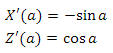
:

? . , ( t >= 0):
X

Y

, (2, 3),
P(t) :

« (3, 2) t (2, 3)». :

X

Y

. : « (3, 2), ».
. , . :
:
? . , ( t >= 0):
X
Y
, (2, 3),
P(t) :
« (3, 2) t (2, 3)». :
X
Y
. : « (3, 2), ».
Appendix 4
F(H), [Hmin, Hmax] 0 1, F(Hmin) = 0 F(Hmax) = 1.
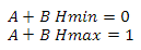
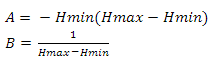
F
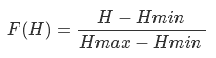
, 0 1 . , — . :
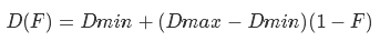


D(F(H))
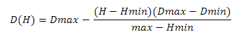
F
, 0 1 . , — . :
D(F(H))
Source: https://habr.com/ru/post/335588/
All Articles