ML Boot Camp V, solution history for 2nd place
In this article, I will tell the story of how the ML Boot Camp V contest “Predicting Cardiovascular Diseases” solved and took second place in it.
Problem statement and data
The data contained 100,000 patients, of which 70% were in the training set, 10% for the public leaderboard (public) and the final 20% (private), on which the result of the competition was determined. The data was the result of a medical examination of patients, based on which it was necessary to predict whether a patient has cardiovascular disease (CVD) or not (this information was available for 70% and it was necessary to predict the probability of CVD for the remaining 30%). In other words, this is a classic binary classification problem. Quality metric - log loss .
The result of the medical examination consisted of 11 signs:
- General - age, gender, height, weight
- Objective - upper and lower pressure, cholesterol level (3 categories: normal, higher than normal) and blood glucose (also 3 categories).
- Subjective - smoking, alcohol, active lifestyle (binary signs)
Since the subjective signs were based on the patient's responses (may be unreliable), the organizers of the competition concealed 10% of each of the subjective signs in the test data. The sample was balanced. Height, weight, upper and lower pressure needed to be cleaned, as they contained typos.
Cross validation
The first important point is correct cross-validation, since the test data had missing data in the smoke, alco, active fields. Therefore, in a validation sample, 10% of these fields were also hidden. Using 7 folds of validation (CV) with a modified validation set, I looked at several different strategies for improving predictions on smoke, alco, active:
- Leave the data in training as it is (in validation 10% of missing values in smoke, alco, active). This approach requires algorithms that can handle missing values (NaN), for example - XGBoost .
- Hide in training 10% so that the training sample is more like validation. This approach also requires algorithms that can work with NaN.
- Predict NaN in validation on three trained classifiers
- Replace signs of smoke, alco, active with predicted probabilities.
The strategy of weighting training examples by proximity to validation / test data was also considered, which, however, did not increase due to the same distribution of train-test.
Hiding in training almost always showed the best CV results, and the optimal share of hidden values in training also turned out to be 10%.
I would like to add that if standard cross-validation is used without hiding values in validation, then CV was obtained better, but overestimated, since the test data in this case is not similar to local validation.
Leaderboard Correlation
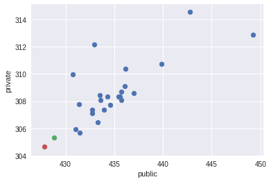
An interesting question that always excites participants is the correlation between the CV and the test data. Already having complete data after the end of the competition (link), I conducted a small analysis of this correlation. For almost all submitters, I wrote down CV results in the description. Having also the result on public and private, we construct pairwise schedules of submits for CV, public, private values (Since all logloss values start at 0.5, for clarity, I omitted the first digits, for example, 370 is 0.5370, and 427.78 - 0.542778):

To get a numerical estimate of the correlation, I chose the Spearman coefficient (others will do as well, but in this case it is the monotonic dependence that is important).
| Spearman rho | CV | Public | Private |
|---|---|---|---|
| CV | one | 0.723 | 0.915 |
| Public | - | one | 0.643 |
| Private | - | - | one |
It can be concluded that the cross-validation introduced in the previous section correlated well with the private for my submissions (during the whole competition), while the public correlation with CV or private is weak.
Small comments: I didn’t sign the CV result for all submitters, and among the CV data there are results with not the best strategies for working with NaN (but the overwhelming majority with the best strategy described in the previous section). Also, these graphs do not contain my two final submissions, which I will discuss below. I depicted them separately in the public-private space with a red and green dot.
Models
During this contest, I used the following models with the appropriate libraries:
- Regularized Gradient Boosting (XGBoost library) is the main model on which I relied, as it showed the best results in my experiments. Also, most of the averages were built on only a few xgb.
- Neural Networks ( Keras library) - experimented with feed forward networks, autoencoders, but it was impossible to beat your baseline from xgb, even in averaging.
- Different sklearn models that participated in averaging with xgb - RF, ExtraTrees, etc.
- Stacking ( brew library) - it was not possible to improve the baseline averaging of several different xgb.
After experimenting with different models and getting the best results by mixing 2-3 xgb (cross-validation took 3-7 minutes), I decided to concentrate more on data cleansing, trait conversion and careful tuning of 1-5 different xgb hyperparameter sets.
I tried to search for hyper parameters using Bayesian optimization (the bayes_opt library), but mostly relied on a random search that served as initialization for Bayesian optimization. Also, in addition to the banal optimal number of trees, after such a search, I tried alternately to pull up the parameters (mainly the regularization parameters of the min_child_weight and reg_lambda trees) —a method that some people call graduate student descent.
Data cleaning I
The first data cleansing option, which was implemented by the participants in one way or another, consisted in the simple application of emission control rules:
- For pressures of 12000 and 1200 - divided by 100 and 10
- Multiply by 10 and 100 for pressures of 10 and 1
- Weight type 25 replaced by 125
- Growth of a type 70 to replace with 170
- If the upper pressure is less than the lower, swap
- If the lower pressure is 0, then replace with the upper minus 40
- etc.
Using a few simple rules for cleaning, I was able to achieve an average CV of ~ 0.5375 and a public ~ 0.5435, which showed quite an average result.
The figures show the sequential processing of extreme values and emissions with the arrival of the cleared values of the upper and lower pressure in the last image.

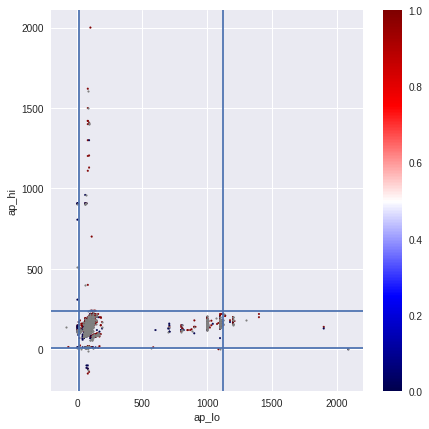
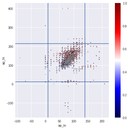

In my experiments, removing emissions did not improve CV.
Data Cleaning II
The previous data cleansing is quite adequate, however, after long attempts at improving the models, I revised it more carefully, which made it possible to significantly improve the quality. Subsequent models with this purge showed an increase in CV to ~ 0.5370 (from ~ 0.5375), public to ~ 0.5431 (from ~ 0.5435).
The basic idea is that there is an exception to every rule. My process of finding such exceptions was rather routine — for a small group (for example, people with upper pressure between 1100 and 2000), I looked at the values in train and test. For most, of course, the “split by 10” rule worked, but there were always exceptions. These exceptions were easier to change separately for examples than to look for the general logic of exceptions. For example, I replaced such pressure from the general pressure group as 1211 and 1620 with 120 and 160.
In some cases, it was possible to correctly handle exceptions, only including information from other fields (for example, on a bundle of upper and lower pressure). Thus, pressures of the form 1/1099 and 1/2088 were replaced with 110/90 and 120/80, and 14900/90 were replaced with 140/90. The most difficult cases, for example, when replacing the pressure of 585 to 85, 701 to 170, 401 to 140.
In difficult, less than unambiguous cases, I checked how corrections are similar to training and test. For example, I replaced the 13/0 case with 130/80, since it is the most likely. For exceptions from the training set, knowledge of the CVD field also helped me.
A very important point is to distinguish the noise from the signal, in this case, a typo from the real anomalous values. For example, after cleaning I left a small group of people with pressure of 150/60 (they have CVD in training, their pressure fits into one of the categories of CVD) or about 90 cm tall with a small weight.
I will add that pressure has cleared the main increase, whereas with height and weight there were a lot of ambiguities (processing of height-weight is also based on the search for exceptions with further application of the general rule).
Using the full dataset laid out after the competition, we find that this cleaning affected 1379 objects in training (1.97%), 194 in public (1.94%), 402 in private (2.01%). Of course, correcting the anomalous values for 2% dataset was not ideal and you can do it better, but even in this case, the largest CV increase was observed. It is worth noting that after cleaning or working with signs, it is necessary to find more optimal hyperparameters of the algorithms.
Work with signs and their discretization
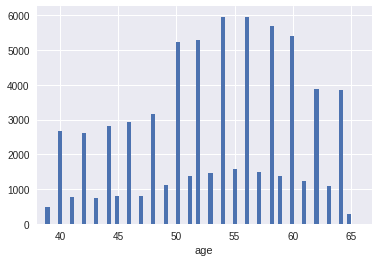
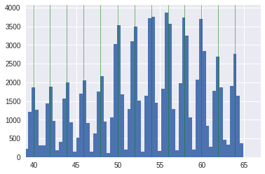
Initially, age was divided by 365.25 to work over the years. The age distribution was periodic, where patients with even years were much more. Age was a Gaussian mixture with 13 centers in even years. If you just round it up by year, then the CV in the fourth digit improved by ~ 1-2 units compared to the initial age. The figures show the transition from the original age to rounded up to a year.

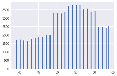
However, I also used a different discretization in order to improve the distribution by years, which I included in the last simple model. The vertices of the distributions in the Gaussian mixture were found using the Gaussian process, and the “year” was defined as half the Gaussian distribution (right and left). Thus, the new distribution by “years” looked more even. The figures show the transition from the initial age (with the found vertices of the Gaussian mixture) to a new distribution over the "years"
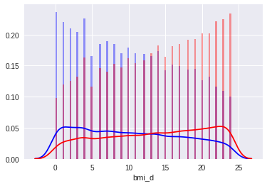
BMI (body mass index = ) appeared first in the importance of signs. Adding the original BMI improved the result; however, the model achieved the greatest improvement after sampling its values. The sampling threshold was chosen on the basis of quartiles, and the number was determined on the basis of cv, visual validation of distributions. The figures show the transition from the original BMI to the discretized BMI.

Similarly, discretization with a small number of categories was applied to height and weight, and pressure and pulse were rounded to an accuracy of 5.
Search for new signs and their selection was done manually. Only a small number of new signs could improve CV, and all of them showed a relatively small increase:
- Pulse pressure - the difference between the upper and lower pressure
- Is the pressure normal (85 <= ap_hi <= 125 & 55 <= ap_lo <= 85)
- The last digit in the pressure before rounding + permutation of the probability of CVD
- Parity analogue of the year (age - (age / 2) .round () * 2)> 0
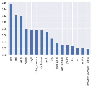
The final importance of features (with discretization) for one xgb model can be seen on the graph:
An hour before the end, I had a rather simple model of 2 xgb using the latest data cleansing and feature sampling. The code is available on github (showed CV 0.5370, public 0.5431, private 0.530569 - also 2nd place).
Last hour of competition
Having averaged two or three xgb on the last data preprocessing, I decided to try to average the results of the latest models with some previous ones (various transformations and feature set, data cleaning, models) and surprisingly, the weights averaging 8 previous predictions gave an improvement to public with 0.5430- 31 to 0.54288. The strategy with weights was fixed immediately - inversely proportional to the rounded 4th digit on the public (for example, 0.5431 weighs 1, 0.5432 - 1/2, 0.5433 - 1/3), which correlated quite well with the fact that the models with the latest data cleansing showed also the best CV values. These 8 predictions were obtained using one, two, three (most), as well as 9 different xgb models. All but one were based on the latest data cleansing, differing in the set of new features, discretization or its absence, hyper-parameters, as well as the strategy with NaN. Further, with the same weighting scheme, adding submits worse (with weights less than 1/4) helped to improve the public to 0.542778 (17 predictions in total, the description can be found on github ).
Of course, it was necessary to keep the results of previous cross-validations in a good way in order to correctly assess the quality of such averaging. Could there be retraining here? Guided by the fact that more than 90% of the weight in averaging was for models with stable CV 0.5370-0.5371, it was possible to expect that the models could help in extreme errors of the best simple models, however, in general, the predictions differed little from the best models. Considering also that the public improved significantly, I chose these two averaging as the final, which resulted in a better model, which showed 2nd place with a private 0.5304688. You may notice that a simple solution, described above, and which was the base in this averaging, would also show 2nd place, but it is less stable.
Lessons learned
The final averaging showed that using a combination of relatively simple models on different features / preprocessing can give better results than using multiple models on the same data. Unfortunately, during the competition I searched for exactly one “ideal” data cleansing, one feature conversion, etc.
Also, for myself, I noticed that in addition to frequent commits in git, it is desirable to store the results of cross-validation of previous models, so that you can quickly assess what mixing of various signs \ preprocessing \ models gives the greatest increase. However, there are exceptions to the rules, for example, if there is only an hour left before the end of the competition.
Judging by the results of other participants, I had to continue my experiments with the inclusion of neural networks, stacking. They, however, were present in my final submission, but only indirectly with little weight.
In conclusion, the presentation of the author is available here , and the presentation is also on github .
')
Source: https://habr.com/ru/post/335226/
All Articles