How to program a satellite photo? Problem solving Dstl Satellite Imagery Feature Detection

Hi, Habr! My name is Yevgeny Nekrasov, I am a research programmer at Mail.Ru Group. Today I will talk about my decision to compete in the data analysis of the Dstl Satellite Imagery Feature Detection , which was dedicated to the segmentation of satellite images. In this competition, I used a relatively simple approach to modeling and took 7th place out of 419 teams. Under the cut - the story of how I did it.

Immediately I will give some introductory, in January 2017, I became the proud owner of the top-end GPU NVIDIA GeForce GTX 1080, and this opened up the opportunity for me to test my theoretical knowledge in Deep Learning on real practical problems. My choice fell on the competition from Dstl on the platform of Kaggle. This task attracted me, firstly, by the unusual data - multispectral satellite images, and secondly, the opportunity to gain valuable practical experience in such an important area as satellite image processing. In this article, the story will be primarily about data analysis techniques and machine learning. Nevertheless, it would be wrong to completely ignore the technical details, so I’ll briefly say that I wrote all the code in Python3 and used the following libraries: numpy, scipy, pandas, skimage, tifffile, shapely, keras with TensorFlow backend.

Formulation of the problem

Data

The organizers provided images of 450 ground pieces 1x1 km. These fragments were from one region of our planet. Each fragment was captured by four WorldView3 satellite sensors: an RGB sensor, a panchromatic sensor, a multispectral sensor, and an SWIR infrared sensor. RGB- and panchromatic sensors, respectively, produce normal color and black-and-white images. What multispectral and SWIR sensors are shown in Fig. 1. Thus, for each fragment 4 TIFF files were given, and they differed both in spatial resolution and dynamic range, the characteristics of the images are shown in Table 1. Of these 450 fragments, 25 were in the training set, to them was provided markup (image segmentation performed by specialists) for 10 classes of objects in the vector format WKT or GeoJSON. The remaining 425 images compiled a test suite, for them it was necessary to build a similar markup for 10 classes in WKT format.
')

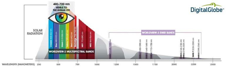
Figure 1. Spectral ranges of a multispectral sensor and a SWIR sensor


Table 1. Characteristics of data from the sensors of the WorldView3 satellite

Now more about 10 classes of objects, these were:

1. Buildings (buildings).
2. Misc. Manmade structures (artificial structures, mainly fences)
3. Road (asphalted roads).
4. Track (dirt roads).
5. Trees (trees).
6. Crops (agricultural fields).
7. Waterway (river).
8. Standing water (small ponds).
9. Vehicle Large (trucks).
10. Vehicle Small (cars).

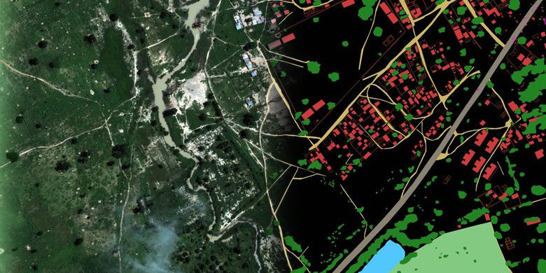
The distribution of the areas of these classes was very uneven on the training marking (Fig. 2). For clarity, here is an example of an RGB image from the training set (Fig. 3) and its markup (Fig. 4).


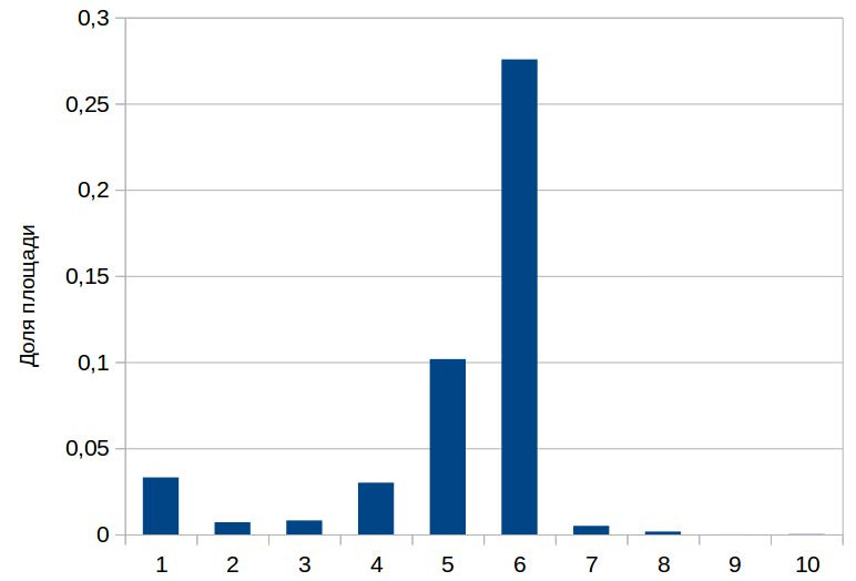
Figure 2. Histogram of shares of areas of classes of objects relative to the total area of ​​the fragment of the earth's surface. 1 - Buildings, 2 - Misc. Manmade structures, 3 - Road, 4 - Track, 5 - Trees, 6 - Crops, 7 - Waterway, 8 - Standing water, 9 - Vehicle Large, 10 - Vehicle Small


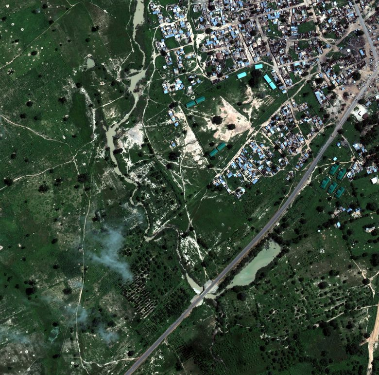
Figure 3. Sample RGB image from the training set


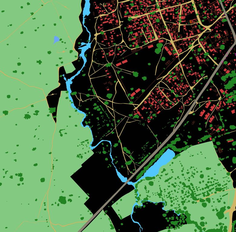
Figure 4. Sample layout from the training set. Red - Buildings, orange - Misc. Manmade structures, gray - Road, yellow - Track, dark green - Trees, light green - Crops, blue - Waterway, blue - Standing water, purple - Vehicle Large, pink - Vehicle Small

The quality metric in the competition was Jaccard (Fig. 5), averaged over all 10 classes. The organizers assessed the quality of the decisions and determined the winners exclusively by this metric, and for the final assessment, which became known only after the competition was over, the organizers used 81% of the test images (Private leaderboard), the remaining 19% of the test images were Public leaderboard and allowed participants to instantly receive preliminary assessment of the quality of their decisions.


Figure 5. An illustration of the Jaccard metric

The solution of the problem

Preprocessing

First you need to bring the data to a form suitable for modeling. I did the preprocessing like this: all four satellite images were scaled to the size of the RGB image (~ 3300x3300 pixels), since it has the highest spatial resolution. Then, each image was normalized to the maximum of the dynamic range, so that the brightness values ​​of the pixels were strictly in the range [0, 1], and then combined into a single 20-channel image. I projected vector marking into raster binary masks, which corresponded in size to a 20-channel image. Transformations of vector marking into raster masks and back I performed using the skimage and shapely libraries.

Modeling

After preprocessing, we get the formulated problem of image segmentation: the training set consists of 25 20-channel images, these images have pixel-by-pixel marking for 10 classes, the test set consists of 425 20-channel images, for which we need to build similar binary masks, which then can be easily converted to vector markup in WKT format - this is what the organizers want.

For the problem of image segmentation, one of the best models is the convolutional neural network of the U-net architecture. The U-net is very similar in structure to the autoencoder, but with one difference: it has the connection of the corresponding parts of the encoder and decoder. The autoencoder part forms a high-level view of the image, and the connections allow the network to effectively segment small parts.

I used two U-net-like artificial neural networks of almost identical architecture (Fig. 6). The first neural network (2c) was sharpened by the segmentation of two extremely rare classes — Vehicle Large and Vehicle Small (Fig. 2). The second neural network (7c) is sharpened for all other classes, and I combined Waterway and Standing water into one class, and there are two reasons for this: first, in fact, Waterway and Standing water are one class - water, and second, There are very few reservoirs in the training set, so it is almost impossible to learn the difference between them from scratch of an artificial neural network, where it is better to divide the already predicted reservoirs into two classes.

The input of both neural networks was 160 by 160 pixels. I got the magic number 160x160 as follows: the larger the field of view of the artificial neural network, the better the neural network can understand the context in which the observed objects are, but with an increase in the neural network, the complexity of the model increases and, accordingly, the time for training and prediction increases. I looked through the satellite images through fields of view of various sizes and realized that the field of view of 160x160 is sufficient to understand the context in this task.


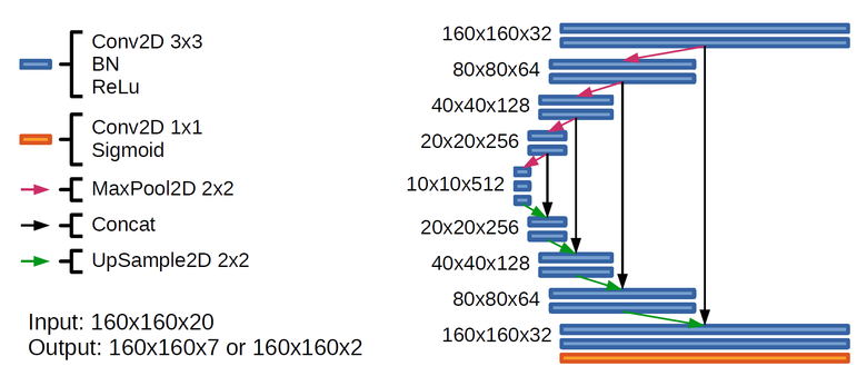
Figure 6. The architecture of neural networks 2c and 7c. In the last layer 7c there were 7 channels at the output, and 2c - 2 channels

Training neural networks

With the training of neural networks in this task, not everything is so simple, because in the training set only 25 images are only about 10 thousand not intersecting image fragments (sprinkles) 160x160 pixels, which is very small and does not allow to fully realize the potential of 2c and 7c networks. Therefore, I used techniques that allow us to solve the problem of a small amount of training data - this is training with partial involvement of the teacher ( semi-supervised learning ) and the expansion of the training set ( data augmentation ). To train both networks, I used binary cross-entropy as a function of loss, that is, taught the network to predict the probability of objects in each pixel, and optimized the weights of neural networks by the Adam optimizer. In the process of training both neural networks, I used training on so-called rotational crocs - image fragments of 160x160 pixels cut from an image with random displacements and turns at a random angle (Fig. 7). This allows us to expand the training set due to our a priori knowledge of the rotational invariance of satellite images, that is, if we rotate the satellite image at an arbitrary angle, then we will get a valid satellite image.


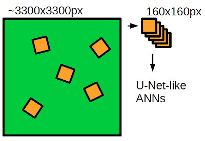
Figure 7. Sample rotation pattern

I will begin the story of the training procedure from the 2c network. Classes of cars and trucks are very rare, so at first I trained a neural network on 200 thousand rotational springs with such a sampling that a car or truck was present in a crop with a probability of about 50%. This was necessary in order for the neural network to get an idea of ​​what constitutes a car or a truck. Then he trained a neural network on 700 thousand rotational spikes with random sampling so that the network would form an adequate idea of ​​the whole dataset as a whole.

For network 7c, I used a more complex approach, applying training with partial involvement of the teacher. The fact is that although we only have 25 marked satellite images at our disposal, we have been given 450 satellite images altogether, and this whole set can be used so that the neural network can learn the concept of what are satellite images in general. I built an autoencoder, which in its structure corresponds to the 7c network and trained it on 600 thousand common crops from all 450 images. Then I transferred the weights of the encoder part of the trained autoencoder into the 7c neural network and fixed them. He trained a network of 400 thousand rotary crop. He released the weights of the encoder part and finished training the neural network for another 600 thousand rotational springs.

Prediction

In order to fulfill the prediction, I traversed the image using a “sliding window”, that is, I cut out 160x160 pixels from the image, performed predictions on them with neural networks 2c and 7c and collected the original image from these fragments. Where it was possible, I used only the central part of the crop predicted by the neural network (Fig. 8) for reconstruction, since the prediction quality is most likely lower at the edges. I performed the “sliding window” passage from each corner of the image, then I averaged the predictions and obtained the final predictions of the probabilities of each class of objects at each point of the image.



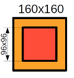
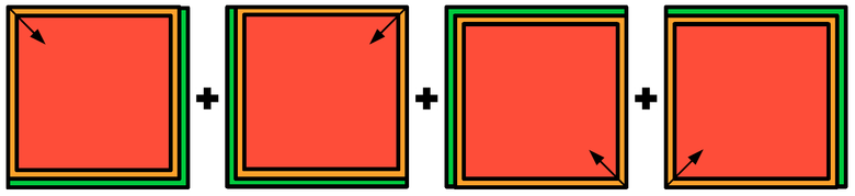
Figure 8. Prediction scheme. Red - predictions from the central cropping area, yellow - predictions from the cropping edge region, green - no predictions

However, we need not probabilities, but binary masks. The easiest way to build them: discretization at the threshold of 0.5. But I used a more advanced method: I performed the prediction on the training set of images, and then I maximized Jaccard on the entire training set relative to the sampling threshold. As a result, we obtained values ​​that often differed significantly from 0.5 (Table 2). The reader may be asked whether there will be retraining here. Neural networks were trained on rotational crocs, and those that were fed into the neural network at the prediction stage could get into the training set with a very small probability, so this is a more or less adequate approach.


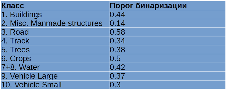
Table 2. Sampling thresholds for different classes of objects

In forming the reservoir prediction, I also used the model for predicting the water of Vladimir Osin , which he laid out in an open access forum of the competition . It is very simple, based on the Canopy Chlorophyl Content Index (CCCI). The index is considered as a combination of the intensity of some channels and allows for the segmentation of water to be efficiently thresholded. I combined my predictions of reservoirs with the results of the work of Vladimir Osin’s model, since these are essentially very different models, and as a result, their combination resulted in a visible improvement in the quality of reservoir segmentation.

Next, it was necessary to divide the predicted water into the Waterway and Standing Water classes. Here I used the classical methods of computer vision and a priori knowledge of the differences between rivers and small ponds. For each area of ​​water, I considered the parameters that should be effective in the separation of these types of water bodies:

• area (rivers are usually larger than ponds by area);
• ellipticity (stretched rivers, ponds close to circumference);
• touching the borders of a photograph (rivers are usually longer than 1 km, and therefore cross the boundaries of a photograph, the probability of being on the boundary of a photograph for a pond is small).

Further, from these parameters I made a linear combination and divided the water classes along the threshold.

So, now we have binary masks for all 10 classes, the problem is solved. Then all that remained was to perform the technical procedures; it was necessary to vectorize the resulting binary masks and save them in the WKT format. I give an example of an image from the test suite (Fig. 9) and its segmentation by the model (Fig. 10).


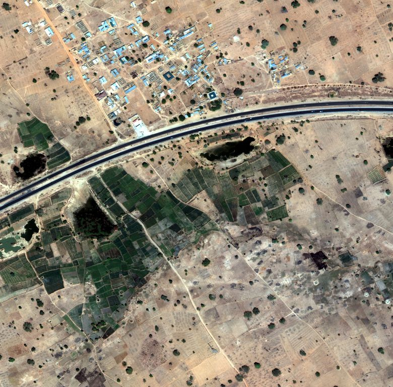
Figure 9. Sample RGB image from the test suite


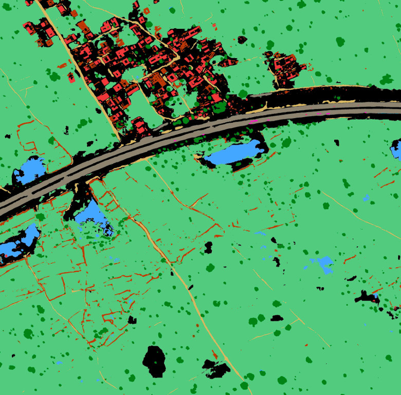
Figure 10. An example of a model prediction in an image from a test suite. Red - Buildings, orange - Misc. Manmade structures, gray - Road, yellow - Track, dark green - Trees, light green - Crops, blue - Waterway, blue - Standing water, purple - Vehicle Large, pink - Vehicle Small

Conclusion

The described solution gives Public Score 0.51725, Private Score 0.43897, and this is the 7th place according to the results of the competition. Here are the key elements of the solution that allowed me to achieve such high results:

1. U-Net architecture, now it’s a state of art for image segmentation.
2. The use of techniques that allowed to work effectively in a small amount of training data. This is training on rotational crocs and the use of test images in the process of learning neural networks.
3. The use of classical methods of computer vision and a priori knowledge for the separation of classes of reservoirs.

This is not a complete list of ideas and approaches that have worked in this competition, you can still learn a lot of interesting ideas from the top published solutions:

• decision of the team of Vladimir Iglovikov and Sergey Mushinsky (3rd place)
• the decision of the team of Roman Solovyov and Artur Kuzin (2nd place)
• Kyle Lee solution (1st place)

Thanks for attention.