Solving a closed transport problem with additional conditions using Python tools
Formulation of the problem
The need to solve transport problems in connection with the territorial disunity of suppliers and consumers is obvious. However, when it is necessary to solve the transportation problem without additional conditions, this is usually not a problem since such solutions are sufficiently well provided both theoretically and with software.
The solution of a closed transport problem by means of Python with classical conditions for suppliers and consumers of the goods is given in my article “Solving linear programming problems using Python” [1].
The real transport problem is complicated by additional conditions and here are some of them. Limited capacity of transport, not taken into account delays in cargo clearance at customs, priorities and parities for suppliers and consumers. Therefore, the solution of a closed transport problem, taking into account additional conditions, has become the goal of this publication.
')
Algorithm for solving a transportation problem with classical conditions
Consider the example of the source data in the form of a table (matrix).
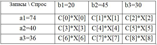
where C = [7,3,6,4,8,2,1,5,5] - a list of the cost of transporting a unit of goods from customers to consumers; X - the list of the volumes of the transported goods, providing the minimum expenses; a = [74,40,36] - a list of volumes of homogeneous goods in the warehouses of suppliers; b = [20,45,30] - a list of volumes demanded by customers of similar goods.
The task is closed because sum (a)> sum (b), therefore for X from the table rows we write the inequalities bounded above, and for X from the columns of the equality table. For further processing, we take the relations in parentheses and equate them to variables.
mass1 = (x [0] + x [1] + x [2] <= 74)
mass2 = (x [3] + x [4] + x [5] <= 40)
mass3 = (x [6] + x [7] + x [8] <= 36
mass4 = (x [0] + x [3] + x [6] == 20
mass5 = (x [1] + x [4] + x [7] == 45)
mass6 = (x [2] + x [5] + x [8] == 30)
The given system of six variables is typical for the transportation problem, it remains to determine the goal function, which, taking into account the list C for the coefficients and variables, will have the form:
problem = op (C [0] * x [0] + C [1] * x [1] + C [2] * x [2] + C [3] * x [3] + C [4] * x [4] + C [5] * x [5] + C [6] * x [6] + C [7] * x [7] + C [8] * x [8], [mass1, mass2, mass3 , mass4, mass5, mass6, x_non_negative])
It should be noted that some solvers have the ability to impose restrictions on all variables X at once, for example, by adding a non-negative –x_non_negative condition to the general conditions.
Formation of additional conditions for the closed transport problem
The reasons for these conditions may be different, for example, the limited capacity of transport, not taking into account delays in processing cargo at customs, priorities and parities for suppliers and consumers. Therefore, we will only indicate the subjects and nature of the restriction.
For further use, we shall number the following additional conditions for the closed transport problem.
1. Installation of a specified volume of delivery of goods from a particular supplier to a specific customer.
To do this, introduce a new variable with the appropriate restriction. For example, the first supplier must supply the second customer exactly 30 units of goods - mass7 = (x [1] == 30) .
2. Change the volume of delivery of goods for a specific customer.
To do this, change the conditions on the column of the table of volumes of deliveries of goods. For example, for the second customer, the order volume decreased from 45 units of goods to 30.
The string of conditions mass5 = (x [1] + x [4] + x [7] == 45) should be replaced by
mass5 = (x [1] + x [4] + x [7] == 30) .
3. Setting the upper limit of the supply of goods for the supplier.
To do this, change the conditions on the line table of the volume of deliveries of goods. For example, for the delivery volumes of the second supplier’s goods there was a top limit <= 40, and it became necessary to deliver exactly 40 units of goods. The condition variable mass2 = (x [3] + x [4] + x [5] <= 40) is replaced by mass2 = (x [3] + x [4] + x [5] == 40) .
4. Parity on deliveries of the second and third suppliers
For this, the supply volumes of several suppliers are equated, which is usually done to improve the business climate. For example, 6 volumes of deliveries of goods from the second and third transport service providers are respectively limited from above <= 40 and <= 36. Replace the lines mass2 = (x [3] + x [4] + x [5] <= 40) and mass3 = (x [6] + x [7] + x [8] <= 36) with mass2 = (x [3] + x [4] + x [5] == 30) and mass3 = (x [6] + x [7] + x [8] == 30) .
Solution of a closed transport problem with additional conditions by means of the cvxopt Python solver
Program for additional condition №1
from cvxopt.modeling import variable, op import time start = time.time() x = variable(9, 'x') c= [7,3,6,4,8,2,1,5,9] z=(c[0]*x[0] + c[1]*x[1] +c[2]* x[2] +c[3]*x[3] + c[4]*x[4] +c[5]* x[5]+c[6]*x[6] +c[7]*x[7] +c[8]* x[8]) mass1 = (x[0] + x[1] +x[2] <= 74) mass2 = (x[3] + x[4] +x[5] <= 40) mass3 = (x[6] + x[7] + x[8] <= 36) mass4 = (x[0] + x[3] + x[6] == 20) mass5 = (x[1] +x[4] + x[7] == 45) mass6 = (x[2] + x[5] + x[8] == 30) mass7 = (x[1] == 30) x_non_negative = (x >= 0) problem =op(z,[mass1,mass2,mass3,mass4 ,mass5,mass6, mass7,x_non_negative]) problem.solve(solver='glpk') print(" Xopt:") for i in x.value: print(i) print(" :") print(problem.objective.value()[0]) stop = time.time() print (" :") print(stop - start) Result hopt:
0.0
30.0
0.0
0.0
0.0
30.0
20.0
15.0
0.0
Cost of delivery:
245.0
Time:
0.04002642631530762
Program for additional condition # 2
from cvxopt.modeling import variable, op import time start = time.time() x = variable(9, 'x') c= [7,3,6,4,8,2,1,5,9] z=(c[0]*x[0] + c[1]*x[1] +c[2]* x[2] +c[3]*x[3] + c[4]*x[4] +c[5]* x[5]+c[6]*x[6] +c[7]*x[7] +c[8]* x[8]) mass1 = (x[0] + x[1] +x[2] <= 74) mass2 = (x[3] + x[4] +x[5] <= 40) mass3 = (x[6] + x[7] + x[8] <= 36) mass4 = (x[0] + x[3] + x[6] == 20) mass5 = (x[1] +x[4] + x[7] == 30) mass6 = (x[2] + x[5] + x[8] == 30) x_non_negative = (x >= 0) problem =op(z,[mass1,mass2,mass3,mass4 ,mass5,mass6,x_non_negative]) problem.solve(solver='glpk') print(" Xopt:") for i in x.value: print(i) print(" :") print(problem.objective.value()[0]) stop = time.time() print (" :") print(stop - start) Result hopt:
0.0
30.0
0.0
0.0
0.0
30.0
20.0
0.0
0.0
Cost of delivery:
170.0
Time:
0.040003299713134766
Program for additional condition No. 3
from cvxopt.modeling import variable, op import time start = time.time() x = variable(9, 'x') c= [7,3,6,4,8,2,1,5,9] z=(c[0]*x[0] + c[1]*x[1] +c[2]* x[2] +c[3]*x[3] + c[4]*x[4] +c[5]* x[5]+c[6]*x[6] +c[7]*x[7] +c[8]* x[8]) mass1 = (x[0] + x[1] +x[2] <= 74) mass2 = (x[3] + x[4] +x[5] == 40) mass3 = (x[6] + x[7] + x[8] <= 36) mass4 = (x[0] + x[3] + x[6] == 20) mass5 = (x[1] +x[4] + x[7] == 45) mass6 = (x[2] + x[5] + x[8] == 30) x_non_negative = (x >= 0) problem =op(z,[mass1,mass2,mass3,mass4 ,mass5,mass6,x_non_negative]) problem.solve(solver='glpk') print(" Xopt:") for i in x.value: print(i) print(" :") print(problem.objective.value()[0]) stop = time.time() print (" :") print(stop - start) Result hopt:
0.0
45.0
0.0
10.0
0.0
30.0
10.0
0.0
0.0
Cost of delivery:
245.0
Time:
0.041509151458740234
Program for additional condition number 4
from cvxopt.modeling import variable, op import time start = time.time() x = variable(9, 'x') c= [7,3,6,4,8,2,1,5,9] z=(c[0]*x[0] + c[1]*x[1] +c[2]* x[2] +c[3]*x[3] + c[4]*x[4] +c[5]* x[5]+c[6]*x[6] +c[7]*x[7] +c[8]* x[8]) mass1 = (x[0] + x[1] +x[2] <= 74) mass2 = (x[3] + x[4] +x[5] == 30) mass3 = (x[6] + x[7] + x[8] == 30) mass4 = (x[0] + x[3] + x[6] == 20) mass5 = (x[1] +x[4] + x[7] == 45) mass6 = (x[2] + x[5] + x[8] == 30) x_non_negative = (x >= 0) problem =op(z,[mass1,mass2,mass3,mass4 ,mass5,mass6,x_non_negative]) problem.solve(solver='glpk') print(" Xopt:") for i in x.value: print(i) print(" :") print(problem.objective.value()[0]) stop = time.time() print (" :") print(stop - start) Result hopt:
0.0
35.0
0.0
0.0
0.0
30.0
20.0
10.0
0.0
Cost of delivery:
235.0
Time:
0.039984941482543945
Solving a closed transport problem with additional conditions by means of the scipy solver. optimize Python
Program for additional condition №1
from scipy.optimize import linprog import time start = time.time() c = [7, 3,6,4,8,2,1,5,9] b_ub = [74,40,36] A_ub = [[1,1,1,0,0,0,0,0,0], [0,0,0,1,1,1,0,0,0], [0,0,0,0,0,0,1,1,1]] b_eq = [20,45,30,30] A_eq = [[1,0,0,1,0,0,1,0,0], [0,1,0,0,1,0,0,1,0], [0,0,1,0,0,1,0,0,1], [0,1,0,0,0,0,0,0,0]] print(linprog(c, A_ub, b_ub, A_eq, b_eq)) stop = time.time() print (" :") print(stop - start) Result:
fun: 245.0
message: 'Optimization terminated successfully.'
nit: 10
slack: array ([44., 10., 1.])
status: 0
success: True
x: array ([0., 30., 0., 0., 0., 30., 20., 15., 0.])
Time:
0.01000523567199707
Program for additional condition # 2
from scipy.optimize import linprog import time start = time.time() c = [7, 3,6,4,8,2,1,5,9] b_ub = [74,40,36] A_ub = [[1,1,1,0,0,0,0,0,0], [0,0,0,1,1,1,0,0,0], [0,0,0,0,0,0,1,1,1]] b_eq = [20,30,30] A_eq = [[1,0,0,1,0,0,1,0,0], [0,1,0,0,1,0,0,1,0], [0,0,1,0,0,1,0,0,1]] print(linprog(c, A_ub, b_ub, A_eq, b_eq)) stop = time.time() print (" :") print(stop - start) Result:
fun: 170.0
message: 'Optimization terminated successfully.'
nit: 7
slack: array ([44., 10., 16.])
status: 0
success: True
x: array ([0., 30., 0., 0., 0., 30., 20., 0., 0.])
Time:
0.04005861282348633
Program for additional condition No. 3
from scipy.optimize import linprog import time start = time.time() c = [7, 3,6,4,8,2,1,5,9] b_ub = [74,36] A_ub = [[1,1,1,0,0,0,0,0,0], [0,0,0,0,0,0,1,1,1]] b_eq = [20,45,30,40] A_eq = [[1,0,0,1,0,0,1,0,0], [0,1,0,0,1,0,0,1,0], [0,0,1,0,0,1,0,0,1], [0,0,0,1,1,1,0,0,0]] print(linprog(c, A_ub, b_ub, A_eq, b_eq)) stop = time.time() print (" :") print(stop - start) Result:
fun: 245.0
message: 'Optimization terminated successfully.'
nit: 8
slack: array ([29., 26.])
status: 0
success: True
x: array ([0., 45., 0., 10., 0., 30., 10., 0., 0.])
Time:
0.04979825019836426
Program for additional condition number 4
from scipy.optimize import linprog import time start = time.time() c = [7, 3,6,4,8,2,1,5,9] b_ub = [74] A_ub = [[1,1,1,0,0,0,0,0,0]] b_eq = [20,45,30,30,30] A_eq = [[1,0,0,1,0,0,1,0,0], [0,1,0,0,1,0,0,1,0], [0,0,1,0,0,1,0,0,1], [0,0,0,1,1,1,0,0,0], [0,0,0,0,0,0,1,1,1]] print(linprog(c, A_ub, b_ub, A_eq, b_eq)) stop = time.time() print (" :") print(stop - start) Result:
fun: 235.0
message: 'Optimization terminated successfully.'
nit: 8
slack: array ([39.])
status: 0
success: True
x: array ([0., 35., 0., 0., 0., 30., 20., 10., 0.])
Time:
0.05457925796508789
Solving a closed transport problem with additional conditions using the pulp Python solver
Program for additional condition №1
from pulp import * import time start = time.time() x1 = pulp.LpVariable("x1", lowBound=0) x2 = pulp.LpVariable("x2", lowBound=0) x3 = pulp.LpVariable("x3", lowBound=0) x4 = pulp.LpVariable("x4", lowBound=0) x5 = pulp.LpVariable("x5", lowBound=0) x6 = pulp.LpVariable("x6", lowBound=0) x7 = pulp.LpVariable("x7", lowBound=0) x8 = pulp.LpVariable("x8", lowBound=0) x9 = pulp.LpVariable("x9", lowBound=0) problem = pulp.LpProblem('0',pulp.LpMaximize) problem += -7*x1 - 3*x2 - 6* x3 - 4*x4 - 8*x5 -2* x6-1*x7- 5*x8-9* x9, " " problem +=x2==30 problem +=x1 + x2 +x3<= 74,"1" problem +=x4 + x5 +x6 <= 40, "2" problem +=x7 + x8+ x9 <= 36, "3" problem +=x1+ x4+ x7 == 20, "4" problem +=x2+x5+ x8 == 45, "5" problem +=x3 + x6+x9 == 30, "6" problem.solve() print (":") for variable in problem.variables(): print (variable.name, "=", variable.varValue) print (" :") print (abs(value(problem.objective))) stop = time.time() print (" :") print(stop - start) Result:
x1 = 0.0
x2 = 30.0
x3 = 0.0
x4 = 0.0
x5 = 0.0
x6 = 30.0
x7 = 20.0
x8 = 15.0
x9 = 0.0
Cost of delivery:
245.0
Time:
0.16973495483398438
Program for additional condition # 2
from pulp import * import time start = time.time() x1 = pulp.LpVariable("x1", lowBound=0) x2 = pulp.LpVariable("x2", lowBound=0) x3 = pulp.LpVariable("x3", lowBound=0) x4 = pulp.LpVariable("x4", lowBound=0) x5 = pulp.LpVariable("x5", lowBound=0) x6 = pulp.LpVariable("x6", lowBound=0) x7 = pulp.LpVariable("x7", lowBound=0) x8 = pulp.LpVariable("x8", lowBound=0) x9 = pulp.LpVariable("x9", lowBound=0) problem = pulp.LpProblem('0',pulp.LpMaximize) problem += -7*x1 - 3*x2 - 6* x3 - 4*x4 - 8*x5 -2* x6-1*x7- 5*x8-9* x9, " " problem +=x1 + x2 +x3<= 74,"1" problem +=x4 + x5 +x6 <= 40, "2" problem +=x7 + x8+ x9 <= 36, "3" problem +=x1+ x4+ x7 == 20, "4" problem +=x2+x5+ x8 == 30, "5" problem +=x3 + x6+x9 == 30, "6" problem.solve() print (":") for variable in problem.variables(): print (variable.name, "=", variable.varValue) print (" :") print (abs(value(problem.objective))) stop = time.time() print (" :") print(stop - start) Result:
x1 = 0.0
x2 = 30.0
x3 = 0.0
x4 = 0.0
x5 = 0.0
x6 = 30.0
x7 = 20.0
x8 = 0.0
x9 = 0.0
Cost of delivery:
170.0
Time:
0.18919610977172852
Program for additional condition No. 3
from pulp import * import time start = time.time() x1 = pulp.LpVariable("x1", lowBound=0) x2 = pulp.LpVariable("x2", lowBound=0) x3 = pulp.LpVariable("x3", lowBound=0) x4 = pulp.LpVariable("x4", lowBound=0) x5 = pulp.LpVariable("x5", lowBound=0) x6 = pulp.LpVariable("x6", lowBound=0) x7 = pulp.LpVariable("x7", lowBound=0) x8 = pulp.LpVariable("x8", lowBound=0) x9 = pulp.LpVariable("x9", lowBound=0) problem = pulp.LpProblem('0',pulp.LpMaximize) problem += -7*x1 - 3*x2 - 6* x3 - 4*x4 - 8*x5 -2* x6-1*x7- 5*x8-9* x9, " " problem +=x1 + x2 +x3<= 74,"1" problem +=x4 + x5 +x6 == 40, "2" problem +=x7 + x8+ x9 <= 36, "3" problem +=x1+ x4+ x7 == 20, "4" problem +=x2+x5+ x8 == 45, "5" problem +=x3 + x6+x9 == 30, "6" problem.solve() print (":") for variable in problem.variables(): print (variable.name, "=", variable.varValue) print (" :") print (abs(value(problem.objective))) stop = time.time() print (" :") print(stop - start) Result:
x1 = 0.0
x2 = 45.0
x3 = 0.0
x4 = 10.0
x5 = 0.0
x6 = 30.0
x7 = 10.0
x8 = 0.0
x9 = 0.0
Cost of delivery:
245.0
Time:
0.17000865936279297
Program for additional condition number 4
from pulp import * import time start = time.time() x1 = pulp.LpVariable("x1", lowBound=0) x2 = pulp.LpVariable("x2", lowBound=0) x3 = pulp.LpVariable("x3", lowBound=0) x4 = pulp.LpVariable("x4", lowBound=0) x5 = pulp.LpVariable("x5", lowBound=0) x6 = pulp.LpVariable("x6", lowBound=0) x7 = pulp.LpVariable("x7", lowBound=0) x8 = pulp.LpVariable("x8", lowBound=0) x9 = pulp.LpVariable("x9", lowBound=0) problem = pulp.LpProblem('0',pulp.LpMaximize) problem += -7*x1 - 3*x2 - 6* x3 - 4*x4 - 8*x5 -2* x6-1*x7- 5*x8-9* x9, " " problem +=x1 + x2 +x3<= 74,"1" problem +=x4 + x5 +x6 == 30, "2" problem +=x7 + x8+ x9 == 30, "3" problem +=x1+ x4+ x7 == 20, "4" problem +=x2+x5+ x8 == 45, "5" problem +=x3 + x6+x9 == 30, "6" problem.solve() print (":") for variable in problem.variables(): print (variable.name, "=", variable.varValue) print (" :") print (abs(value(problem.objective))) stop = time.time() print (" :") print(stop - start) Result:
x1 = 0.0
x2 = 35.0
x3 = 0.0
x4 = 0.0
x5 = 0.0
x6 = 30.0
x7 = 20.0
x8 = 10.0
x9 = 0.0
Cost of delivery:
235.0
Time:
0.17965340614318848
Conclusion
The additional conditions obtained in the publication for a closed transport problem allow one to obtain solutions that are more close to the actual situation with the delivery of goods. The above additions can be used in several ways in one task, applying them depending on the situation. The question of choosing a solver for a transportation problem with conditions is investigated. Such a solver is scipy. optimize, as more narrowly functional than cvxopt and faster than pulp. Also, scipy. optimize has a more compact record of the conditions of the transport problem, which facilitates its work with the interface.
Thank you all for your attention!
Links
Source: https://habr.com/ru/post/335104/
All Articles