TSP problem. Mixed algorithm
Good day to all. In previous articles, we compared two heuristic optimization algorithms on a symmetric traveling salesman problem such as: ACS (ant colony system - ant algorithm) and SA (simulating annealing - annealing simulation algorithm). As we have seen each has its own pros and cons.

The advantages of SA are the relatively high speed of the algorithm, the ease of implementation. Of the minuses - the algorithm is not "flexible", there is also no so-called "ability to rebuild the figure." For those who want to grasp the essence of the simulation annealing algorithm, refer to this article .
Pros AS (ACS) - the presence of collectivism, the convergence of the algorithm from iteration to iteration, the ability to rebuild the figure (always looking for alternative ways, in fact, with the correct selection of parameters does not get stuck on the local optimum), the possibility of partial parallelism. Of the minuses - a long time algorithm, the complexity of a high number of vertices. Those who want to grasp the essence of the ant algorithm refer to the site . You can also see the code written in MatLab in my previous articles; there you can understand the principle in the comments.
Today I would like to show you the first version of the algorithm, which has absorbed the best of different algorithms, and which is able to find, from the first attempt with a high probability, a global optimal path to 100 vertices in less than 5 seconds on a regular home PC. I will try to show everything by examples with graphic illustrations. The code is written in MatLab. Mostly in his element - vector, if anyone has problems with the transfer of the algorithm to your language - write in the comments. Those who are interested more seriously, or those who want to implement their version - I suggest to look at previous articles, and also to see the full code of the algorithm, which will be attached below the article. In the comments I tried to paint every line.
')
Immediately, I note that this algorithm may already exist, but I did not find it in the vastness of the global network. So, how should it be in the implementation of this article:
1 - as simple as possible
2 - The fastest
3 - The possibility of parallelization on the CPU (including the current fashionable GPU)
4 - Flexible (possibility of upgrading, variability of parameters)
5 - Less dependent on random parameters.
6 - Ability to rebuild the figure
By what I mean rebuilding the figure, see below.
Rebuilding a TSP shape on task Eil101 (traveling salesman problem):
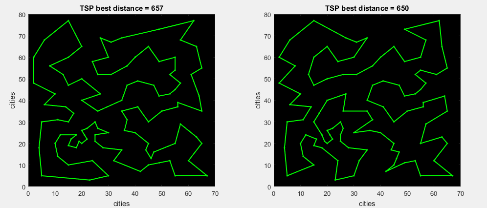
The image shows that the distance of both routes differs by 1%, but their routes are completely different. That is completely different figures. A good algorithm should create as many similar shapes as possible. In SA it is poorly developed.
The method of simulating annealing (as we have seen in previous articles) at the initial high temperature, as well as at a slowly falling temperature, is able to achieve good results, but this significantly increases the algorithm time, nor does it guarantee that the global best path will be found. It’s another thing if we run several SA algorithms at once, add the results of each to the array and select the best one.
One of the drawbacks of the classic SA algorithm is that there are too many “randoms” in it, first we randomly select two vertices, then again “random”, in order to make or not make the worst decision. In this algorithm, I tried to minimize the proportion of chance.
Therefore, in this algorithm, instead of “randomizing” two vertices, we immediately iterate over all possible parts of the inversion path. Let me remind you that our goal is only the global optimum, onlyhardcore . More precisely not global, but the best found to date.
Clarification:
There is a route: [1,2,3,4,5,6,7,8] - the traveler first visits the first city, then the second, etc. “Random two vertices” means randomly choosing two numbers (even distribution), say 2 and 6, then invert the path between them. The path will take the form: [1, 6 , 5,4,3, 2 , 8].
We completely enumerate the parts of the path inversion into a function that accepts a route (any, even the most incorrect one), searches for the most profitable part of the route for a turn, unfolds it, then again searches for the most profitable part of the route taking into account the previous changes and repeats the cycle until , while no replacement of part of the route will improve the distance.
This method is known as the 2opt algorithm. However, in the classic 2opt algorithm, we immediately expand a part of the route, which improves the result, but here we are looking for, in addition to the standard 2opt, also the “best replacement”.
Graphic illustration:
on the 1st gif animation, the algorithm immediately expands the found part of the route, which improves the total distance (standard 2-opt)
on the 2nd gif animation, the algorithm drives all possible replacements of a part of the route, then expands the most maximal delta (m. 2-opt)
In today's algorithm, we will use the second option, since in a series of tests it shows far better results. The first option will be left for revision.
So, we have two functions that optimize the route with a kind of "modernized method of simulating annealing." It remains only to pass by a parallel loop (in MatLabe, the parfor operator allows you to use all the cores of a PC) into the function a couple of thousand of such routes (which will also be created by a parallel loop) and select the best one.
This is where the fun begins.
What routes to transmit? Naturally, when exiting, they should contain as many different figures as possible (see above). Also, if we simply transmit a random array, then we will not see the best result globally. So let our array of routes to the input of the function “all_brute_best” consist of different algorithms.
The first that immediately came to mind is the method of the nearest neighbor . We will leave each city once, and get an array of nxn routes (n is the number of cities). Then we transfer this array to the optimization function.
At Matlabe, the nearest city will be visited as follows:
In general, TSP tasks (traveling salesman problem) were solved by many. They were also solved by the most “hard-boiled” algorithms. So on the site laid out the best solutions found today.
Let us check the algorithm on the problem Eil76, the visual work of which is presented below. The best path found is 538.
After completing all 76 optimizations, we get the best route found - 545. The elapsed time is 0.15 seconds. This algorithm will always find the distance in 545, since there is no share of randomness in it. The global error is 1.3%.
Now the fun part. As you probably noticed, we just mixed the greedy algorithm, brute force (brute force) and imitation annealing. Now it's time to add some ant algorithm. Now, in our algorithm, before transferring to the optimization function, the transition to the nearest city is performed with a 100% probability. Our task is to find the best route found, make up as many “figures” as possible and pass them to the function. As we remember from the ant algorithm (AS), the probability of transition from vertex i to vertex j is determined by the following formula:
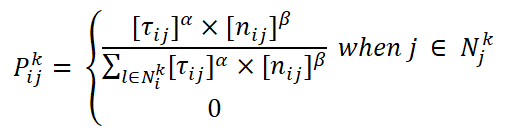
where [τ (i, j)] is the pheromone level on the edge (i, j), [n (i, j)] is the weight inverse to the distance on the edge (i, j), β is an adjustable parameter, the higher it is, the the algorithm will tend to select an edge that has a shorter distance. Since there are no pheromones in this algorithm, we remove them. Leave only the level of "greed" algorithm. We carry, as in ACS, the probability of choosing an unvisited vertex. Either we select only the shortest city, or proceed as follows:
The probability of choosing the next edge will be inversely proportional to its length. We also introduce the variable responsible for the selection of cities that have not yet been visited. That is, when choosing the next vertex, we will not take into account all the remaining ones, but we will choose among the N-th number of the remaining peaks. N is a user defined parameter. This idea was taken from the genetic algorithm. In the genetic algorithm there is the concept of “selection”, at the stage of which it is necessary to select a certain share from the entire current population, which will remain “to live”. The probability of survival of an individual should depend on the value of the function of fitness. Here, the value of the function of fitness is the distance of the edge, and the population is the share of the remaining cities not visited. We simply choose only one “individual” from the whole population, i.e. one vertex. The formula for the probability of taking the next edge will be:
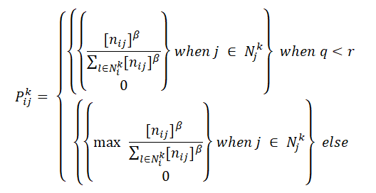
where q is the probability of making an alternative decision (not necessarily the shortest edge)
r is a random number [0; 1]
N - edges involved in the selection (sortable)
Thus, we will form a set of "controlled" different routes to the input of the all_brute function. The word controlled means the control of randomness of the route. The more the q parameter tends to 1, just as the N tends to the total number of cities, the more random the search will be.
So, we look at the results on various tasks:
Exact solutions:
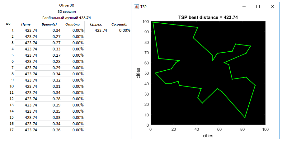
Oliver30 task (30 vertices). Global best way - 423.741
Parameters: the number of created routes to enter - 500
q = 0.03
N = 10
Problem Eil51 (51 vertices). Global best way - 426
Parameters: the number of routes created for entry - 2500
q = 0.03
N = 5

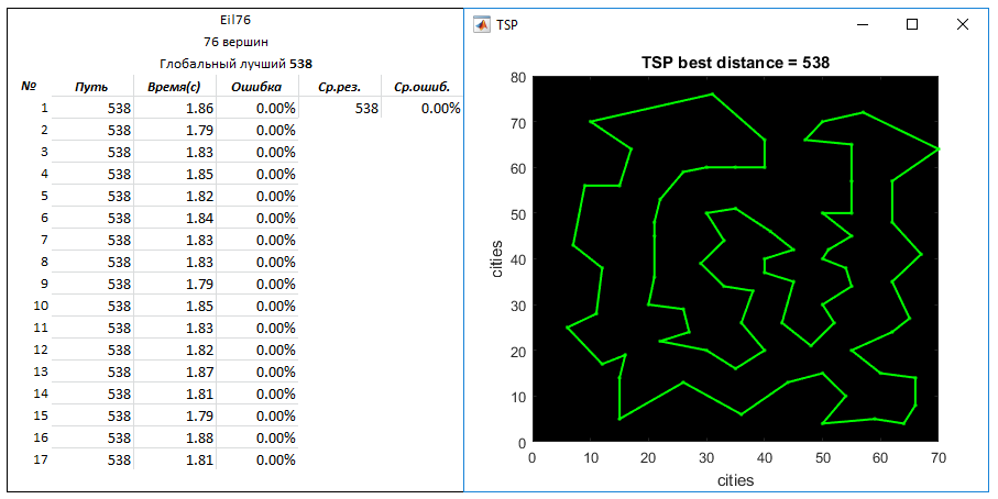
Problem Eil76 (76 vertices). Global best way - 538
Parameters: the number of generated routes to the entrance - 4000
q = 0.03
N = 10
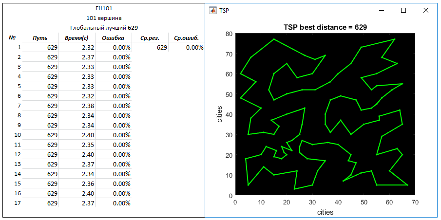
Problem Eil101 (101 vertices). Global Best Way - 629
Parameters: the number of routes created for entry - 2500
q = 0.03
N = 6
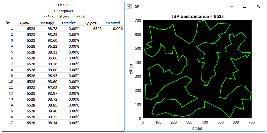
Ch150 problem (150 vertices). Global Best Way - 6528
Parameters: the number of generated routes to the entrance - 40000
q = 0.05
N = 10
The result was good. Yes, this algorithm is much more efficient than heuristic algorithms, such as an annealing simulation method or a genetic algorithm. But agree that the range of problem solving by the genetic algorithm is extremely wide, which cannot be said about this algorithm. However, it was interesting to find out the result when mixing different algorithms.
The main goal of this algorithm is to create an array of optimized routes, as well as their distance array. In the next article, we, using this array, will combine the genetic and ant algorithms. We enable computing on the GPU. And we will aim at finding a global best path of 500, 1000 and 2000 vertices on a home PC in a very reasonable time. Looking ahead to say that it is quite real.
So, in this article we found the best paths found so far in various tasks. The huge gap between the best found ever and the approximate solution. If this algorithm finds approximate solutions, then the execution time of the algorithm will be 10 times lower.
Below is the main code of the algorithm with comments (its functions were published above)
Thanks for attention. Until new meetings.
The advantages of SA are the relatively high speed of the algorithm, the ease of implementation. Of the minuses - the algorithm is not "flexible", there is also no so-called "ability to rebuild the figure." For those who want to grasp the essence of the simulation annealing algorithm, refer to this article .
Pros AS (ACS) - the presence of collectivism, the convergence of the algorithm from iteration to iteration, the ability to rebuild the figure (always looking for alternative ways, in fact, with the correct selection of parameters does not get stuck on the local optimum), the possibility of partial parallelism. Of the minuses - a long time algorithm, the complexity of a high number of vertices. Those who want to grasp the essence of the ant algorithm refer to the site . You can also see the code written in MatLab in my previous articles; there you can understand the principle in the comments.
Today I would like to show you the first version of the algorithm, which has absorbed the best of different algorithms, and which is able to find, from the first attempt with a high probability, a global optimal path to 100 vertices in less than 5 seconds on a regular home PC. I will try to show everything by examples with graphic illustrations. The code is written in MatLab. Mostly in his element - vector, if anyone has problems with the transfer of the algorithm to your language - write in the comments. Those who are interested more seriously, or those who want to implement their version - I suggest to look at previous articles, and also to see the full code of the algorithm, which will be attached below the article. In the comments I tried to paint every line.
')
Immediately, I note that this algorithm may already exist, but I did not find it in the vastness of the global network. So, how should it be in the implementation of this article:
1 - as simple as possible
2 - The fastest
3 - The possibility of parallelization on the CPU (including the current fashionable GPU)
4 - Flexible (possibility of upgrading, variability of parameters)
5 - Less dependent on random parameters.
6 - Ability to rebuild the figure
By what I mean rebuilding the figure, see below.
Rebuilding a TSP shape on task Eil101 (traveling salesman problem):
The image shows that the distance of both routes differs by 1%, but their routes are completely different. That is completely different figures. A good algorithm should create as many similar shapes as possible. In SA it is poorly developed.
The method of simulating annealing (as we have seen in previous articles) at the initial high temperature, as well as at a slowly falling temperature, is able to achieve good results, but this significantly increases the algorithm time, nor does it guarantee that the global best path will be found. It’s another thing if we run several SA algorithms at once, add the results of each to the array and select the best one.
One of the drawbacks of the classic SA algorithm is that there are too many “randoms” in it, first we randomly select two vertices, then again “random”, in order to make or not make the worst decision. In this algorithm, I tried to minimize the proportion of chance.
Therefore, in this algorithm, instead of “randomizing” two vertices, we immediately iterate over all possible parts of the inversion path. Let me remind you that our goal is only the global optimum, only
Clarification:
There is a route: [1,2,3,4,5,6,7,8] - the traveler first visits the first city, then the second, etc. “Random two vertices” means randomly choosing two numbers (even distribution), say 2 and 6, then invert the path between them. The path will take the form: [1, 6 , 5,4,3, 2 , 8].
We completely enumerate the parts of the path inversion into a function that accepts a route (any, even the most incorrect one), searches for the most profitable part of the route for a turn, unfolds it, then again searches for the most profitable part of the route taking into account the previous changes and repeats the cycle until , while no replacement of part of the route will improve the distance.
This method is known as the 2opt algorithm. However, in the classic 2opt algorithm, we immediately expand a part of the route, which improves the result, but here we are looking for, in addition to the standard 2opt, also the “best replacement”.
Graphic illustration:
on the 1st gif animation, the algorithm immediately expands the found part of the route, which improves the total distance (standard 2-opt)
on the 2nd gif animation, the algorithm drives all possible replacements of a part of the route, then expands the most maximal delta (m. 2-opt)
In today's algorithm, we will use the second option, since in a series of tests it shows far better results. The first option will be left for revision.
So, we have two functions that optimize the route with a kind of "modernized method of simulating annealing." It remains only to pass by a parallel loop (in MatLabe, the parfor operator allows you to use all the cores of a PC) into the function a couple of thousand of such routes (which will also be created by a parallel loop) and select the best one.
Brute force function (best replacement)
% % ( ) % dist - % route - % openclose - %------------------------------------------------------------------------ function [tour, distance] = all_brute_best(dist,route,n) global_diff = -0.1; best_dist = inf; % , while global_diff < 0 global_diff = 0; p1 = route(n); % for i = 1:n-2 t1 = p1; p1 = route(i); t2 = route(i+1); spd_var = dist(t1,p1); for j = i+2:n p2 = t2; t2 = route(j); diff = (dist(t1,p2) - dist(p2,t2))... + (dist(p1,t2) - spd_var); % if global_diff > diff global_diff = diff; % "" imin = i; jmin = j; end end end % if global_diff < 0 route(imin:jmin-1) = route(jmin-1:-1:imin); end end %-------------------------------------------------------------------- % cur_dist = 0; for i = 1:n-1 cur_dist = cur_dist + dist(route(i),route(i+1)); end % cur_dist = cur_dist + dist(route(1),route(end)); %-------------------------------------------------------------------- % if cur_dist < best_dist best_route = route; best_dist = cur_dist; end % - distance = best_dist; % tour = best_route; end Brute force function (each replacement)
% % ( ) % dist - % route - % openclose - %------------------------------------------------------------------------- function [tour, distance] = all_brute_first(dist,route,n) global_diff = -0.1; best_dist = inf; % , while global_diff < 0 global_diff = 0; p1 = route(n); % for i = 1:n-2 t1 = p1; p1 = route(i); t2 = route(i+1); spd_var = dist(t1,p1); for j = i+2:n p2 = t2; t2 = route(j); diff = (dist(t1,p2) - dist(p2,t2))... + (dist(p1,t2) - spd_var); % if diff < 0 global_diff = diff; % "" imin = i; jmin = j; break end end % if diff < 0 break end end % if global_diff < 0 route(imin:jmin-1) = route(jmin-1:-1:imin); end end %-------------------------------------------------------------------- % cur_dist = 0; for i = 1:n-1 cur_dist = cur_dist + dist(route(i),route(i+1)); end % cur_dist = cur_dist + dist(route(1),route(end)); %-------------------------------------------------------------------- % if cur_dist < best_dist best_route = route; best_dist = cur_dist; end % - distance = best_dist; % tour = best_route; end This is where the fun begins.
What routes to transmit? Naturally, when exiting, they should contain as many different figures as possible (see above). Also, if we simply transmit a random array, then we will not see the best result globally. So let our array of routes to the input of the function “all_brute_best” consist of different algorithms.
The first that immediately came to mind is the method of the nearest neighbor . We will leave each city once, and get an array of nxn routes (n is the number of cities). Then we transfer this array to the optimization function.
At Matlabe, the nearest city will be visited as follows:
Nearest Neighbor Method
parfor k = 1:n % ( ) dist_temp = dist; % route = zeros(1,n); % next_point = start_route(k); % route(1) = next_point; % for e = 2:n % dist_temp(next_point,:) = nan; % [~,next_point] = min(dist_temp(:,next_point)); % route(e) = next_point; end % 1- if check_routes == true route = check_tour(route); end % arr_route_in(k,:) = route; end In general, TSP tasks (traveling salesman problem) were solved by many. They were also solved by the most “hard-boiled” algorithms. So on the site laid out the best solutions found today.
Let us check the algorithm on the problem Eil76, the visual work of which is presented below. The best path found is 538.
After completing all 76 optimizations, we get the best route found - 545. The elapsed time is 0.15 seconds. This algorithm will always find the distance in 545, since there is no share of randomness in it. The global error is 1.3%.
Now the fun part. As you probably noticed, we just mixed the greedy algorithm, brute force (brute force) and imitation annealing. Now it's time to add some ant algorithm. Now, in our algorithm, before transferring to the optimization function, the transition to the nearest city is performed with a 100% probability. Our task is to find the best route found, make up as many “figures” as possible and pass them to the function. As we remember from the ant algorithm (AS), the probability of transition from vertex i to vertex j is determined by the following formula:
where [τ (i, j)] is the pheromone level on the edge (i, j), [n (i, j)] is the weight inverse to the distance on the edge (i, j), β is an adjustable parameter, the higher it is, the the algorithm will tend to select an edge that has a shorter distance. Since there are no pheromones in this algorithm, we remove them. Leave only the level of "greed" algorithm. We carry, as in ACS, the probability of choosing an unvisited vertex. Either we select only the shortest city, or proceed as follows:
The probability of choosing the next edge will be inversely proportional to its length. We also introduce the variable responsible for the selection of cities that have not yet been visited. That is, when choosing the next vertex, we will not take into account all the remaining ones, but we will choose among the N-th number of the remaining peaks. N is a user defined parameter. This idea was taken from the genetic algorithm. In the genetic algorithm there is the concept of “selection”, at the stage of which it is necessary to select a certain share from the entire current population, which will remain “to live”. The probability of survival of an individual should depend on the value of the function of fitness. Here, the value of the function of fitness is the distance of the edge, and the population is the share of the remaining cities not visited. We simply choose only one “individual” from the whole population, i.e. one vertex. The formula for the probability of taking the next edge will be:
where q is the probability of making an alternative decision (not necessarily the shortest edge)
r is a random number [0; 1]
N - edges involved in the selection (sortable)
Thus, we will form a set of "controlled" different routes to the input of the all_brute function. The word controlled means the control of randomness of the route. The more the q parameter tends to 1, just as the N tends to the total number of cities, the more random the search will be.
Route Build Function
% (probability several route) % , % dist - % tour_sev - - % n - - % tour_select - - % check_routes - % p_change - %------------------------------------------------------------------------- function [arr_several_route] = psr(dist,tour_sev,n,tour_select,cr,p_change) % () arr_several_route = zeros(tour_sev,n); parfor k = 1:tour_sev % ( ) dist_temp = dist; % route = zeros(1,n); % ( ) next_point = randi([1,n]); % route(1) = next_point; % count_var = 0; % for e = 2:n % dist_temp(next_point,:) = nan; % count_var = count_var + 1; % if rand(1) > p_change % k- % [~,next_point] = min(dist_temp(:,next_point)); else % % () arr_next = 1./(dist_temp(:,next_point)); % % , "habrahabr_vis" habrahabr_vis = (1:1:n)'; % arr_next = [arr_next, habrahabr_vis]; % arr_next_sort = sortrows(arr_next,1); % rand if (n - count_var) < tour_select tour_select_fun = (n - count_var); else tour_select_fun = tour_select; end % P = arr_next_sort(1:tour_select_fun,:); P(:,1) = P(:,1)./sum(P(:,1)); randNumb = rand; next_point = P(find(cumsum(P) >= randNumb, 1, 'first'),2); end % route(e) = next_point; end % 1- if cr == true route = check_tour(route); end % ( ) arr_several_route(k,:) = route; end So, we look at the results on various tasks:
Exact solutions:
Oliver30 task (30 vertices). Global best way - 423.741
Parameters: the number of created routes to enter - 500
q = 0.03
N = 10
Problem Eil51 (51 vertices). Global best way - 426
Parameters: the number of routes created for entry - 2500
q = 0.03
N = 5
Problem Eil76 (76 vertices). Global best way - 538
Parameters: the number of generated routes to the entrance - 4000
q = 0.03
N = 10
Problem Eil101 (101 vertices). Global Best Way - 629
Parameters: the number of routes created for entry - 2500
q = 0.03
N = 6
Ch150 problem (150 vertices). Global Best Way - 6528
Parameters: the number of generated routes to the entrance - 40000
q = 0.05
N = 10
The result was good. Yes, this algorithm is much more efficient than heuristic algorithms, such as an annealing simulation method or a genetic algorithm. But agree that the range of problem solving by the genetic algorithm is extremely wide, which cannot be said about this algorithm. However, it was interesting to find out the result when mixing different algorithms.
The main goal of this algorithm is to create an array of optimized routes, as well as their distance array. In the next article, we, using this array, will combine the genetic and ant algorithms. We enable computing on the GPU. And we will aim at finding a global best path of 500, 1000 and 2000 vertices on a home PC in a very reasonable time. Looking ahead to say that it is quite real.
So, in this article we found the best paths found so far in various tasks. The huge gap between the best found ever and the approximate solution. If this algorithm finds approximate solutions, then the execution time of the algorithm will be 10 times lower.
Below is the main code of the algorithm with comments (its functions were published above)
Main
% TSP() ( ) %------------------------------------------------------------------------% if exist('cities','var') == 1 clearvars -except cities n = length(cities(:,1)); else clearvars intvar = inputdlg({'- '}... ,'TSP',1); n = str2double(intvar(1)); if isnan(n) || n < 0 msgbox ' ' return else cities = rand(n,2)*100; end end % tic %---------------------------------------------------------------% % ( x y ) start_tour = 1; % , % ( ) check_routes = false; % roulete_method = false; % (- ) if roulete_method == true crrm = 1000; end % "ts" top_roulete_method = true; if top_roulete_method == true % - " " ctrrm = 1000; % ts = 10; % p_change = 0.05; end %------------------------------------------------------------------% % dist = zeros(n,n); % () best_dist = inf; % brute_edge arr_route_in = zeros(n,n); % - ( ) % b = 1; %------------------------------------------------------------------------% % for i = 1:n for j = 1:n dist(i,j) = sqrt((cities(i,1) - cities(j,1))^2 + ... (cities(i,2) - cities(j,2))^2); end end % dist = round(dist); % returndist = 1./dist; % ( ) start_route = linspace(1,n,n); % if start_tour > n || start_tour < 1 start_tour = 1; end % "start_tour" start_route(start_tour) = 1; start_route(1) = start_tour; % % % parfor - parfor k = 1:n % ( ) dist_temp = dist; % route = zeros(1,n); % next_point = start_route(k); % route(1) = next_point; % for e = 2:n % dist_temp(next_point,:) = nan; % [~,next_point] = min(dist_temp(:,next_point)); % route(e) = next_point; end % 1- if check_routes == true route = check_tour(route); end % arr_route_in(k,:) = route; end % ( ) % if top_roulete_method == true arr_several = psr(dist,ctrrm,n,ts,check_routes,p_change); arr_route_in = [arr_route_in; arr_several]; end % % if roulete_method == true % , [randRoute] = prr(returndist,crrm,n,check_routes); % arr_route_in = [arr_route_in;randRoute]; end % % % parfor r = 1:size(arr_route_in, 1); % temp_route = arr_route_in(r,:); % [~,numb_ix] = find(temp_route == 1); % if numb_ix ~= 1 % temp_route = [temp_route(numb_ix:end),temp_route(1:numb_ix-1)]; % elseif numb_ix == n % temp_route = fliplr(temp_route); % end % arr_route_in(r,:) = temp_route; % end % , arr_route_in = unique(arr_route_in,'rows'); %------------------------------------------------------------------% % () arr_tour_out = zeros(size(arr_route_in,1),n); % () arr_result = zeros(size(arr_route_in,1),1); %------------------------------------------------------------------------% % ( ) spdvar = size(arr_route_in, 1); parfor i = 1:spdvar % [tour, distance] = all_brute_first(dist,arr_route_in(i,:),n); [tour, distance] = all_brute_best(dist,arr_route_in(i,:),n); arr_tour_out(i,:) = tour; arr_result(i,1) = distance; end % toc % [best_length,best_indx] = min(arr_result); % 1- best_route = arr_tour_out(best_indx,:); % % % mean(arr_result) %-----------------------------------------------------------------% tsp_plot = figure(1); set(tsp_plot,'name','TSP','numbertitle','off'... ,'color','w','menubar','none') set(gcf,'position',[2391 410 476 409]); opt_tour(:,[1,2]) = cities(best_route,[1,2]); plot([opt_tour(:,1);opt_tour(1,1)],[opt_tour(:,2);opt_tour(1,2)],'-g.', ... 'linewidth',1.5) set(gca,'color','k') title(['TSP best distance = ',num2str(round(best_length,2))]) xlabel('cities'); ylabel('cities') %------------------------------------------------------------------------% fprintf('%s %d\n',' ',round(best_length)); clearvars -except cities arr_result arr_tour_out arr_route_in ... n best_length opt_tour dist openclose Thanks for attention. Until new meetings.
Source: https://habr.com/ru/post/335016/
All Articles