R from H2O to Spark in HDInsight
 H2O is a machine learning library designed both for local computing and using clusters created directly using H2O or working on a Spark cluster. Integration of H2O into Spark clusters created in Azure HDInsight has been added recently and in this publication (which is an addition to my previous article: R and Spark ), we consider building machine learning models using H2O on such a cluster and compare (time, metric) it with the models provided sparklyr , is H2O a killer app for Spark ?
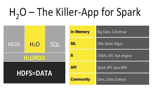
Overview of H20 features in the HDInsight Spark cluster
As mentioned in the previous post, at that time there were three ways to build MO models using R on a Spark cluster, let me remind you:
1) The sparklyr package, which offers different ways to read from various data sources, convenient dplyr data manipulation and a fairly large set of different models.
2) R Server for Hadoop , software from Microsoft , using its functions for data manipulation and its implementation of MO models.
3) The SparkR package, which offers its own implementation of data manipulations and offered a small number of MO models (currently, in the Spark 2.2 version, the list of models has been significantly expanded).
Details of the functionality of each option can be found in Table 1 of the previous post.
Now there is a fourth way - to use H2O in clusters of Spark HDInsight . Consider briefly its capabilities:
- Read-write, data manipulation - they are not directly in H2O, it is necessary to transfer (convert) the finished data from Spark to H20 .
- Machine learning models are slightly smaller than in sparklyr, but all the main ones are available, here is their list:
- Generalized Linear Model
- Multilayer Perceptron
- Random forest
- Gradient Boosting Machine
- Naive-bayes
- Principal Components Analysis
- Singular value decomposition
- Generalized Low Rank Model
- K-Means Clustering
- Anomaly Detection via Deep Learning Autoencoder.
- Additionally, you can use ensembles and stacking several models using the h2oEnsemble package.
- The convenience of H2O models is that it is possible to immediately evaluate the quality metrics, both on the training and on the validation sample.
- Adjustment of hyperparameters of algorithms using a fixed grid or random selection.
- The resulting models can be saved in a binary form or in pure Java code " Plain Old Java Object ". ( POJO )
In general, the algorithm for working with H2O is as follows:
- Reading data using the sparklyr package.
- Manipulation, transformation, data preparation using sparklyr and replyr .
- Convert data to H2O format using rsparkling package.
- MO model building and data prediction using h2o .
- Return the results to Spark and / or locally to R using rsparkling and / or sparklyr .
Resources used
- H2O Artificial Intelligence Cluster for HDInsight 2.0.2.
This cluster is a complete solution with API for Python and Scala . R (apparently so far) is not integrated, but adding it is not difficult, for this you need the following: - R and packages sparklyr , h2o , rsparkling install on all nodes: head and working
- RStudio install on the head node
- putty client locally to establish an ssh session with the cluster head node and tunnel the RStudio port to the local host port to access RStudio via a web browser.
Important: install the h2o package from source, choosing the version corresponding to the version of both Spark and rsparkling , if necessary, before downloading rsparkling, you must specify the version of sparklingwater used (in this case, options (rsparkling.sparklingwater.version = '2.0.8' . The table with dependencies by version is shown here . Installing software and packages on the head nodes is permissible directly through the node console, but there is no direct access to the working nodes, therefore, deployment of additional software must be done through Action Script .
First, we deploy the H2O Artificial Intelligence for HDInsight cluster , the configuration is the same with 2 D12v2 head nodes and 4 D12v2 work nodes and 1 Sparkling water node (service). After successfully deploying the cluster, using the ssh connection to the head node, install R , RStudio (the current version of RStudio already with integrated capabilities for viewing Spark frames and cluster status), and the necessary packages. To install packages on working nodes, create an installation script (R and packages) and initiate it via Action Script . It is possible to use ready-made scripts that are located here: on the head nodes and on the working nodes . After all successful installations, we reinstall the ssh connection using tunneling to localhost: 8787 . So, now in the browser at localhost: 8787 we connect to RStudio and continue to work.
The advantage of using R lies in the fact that having installed a Shiny server on the same parent node and, having created a simple web interface on a flexdashboard , all calculations on the cluster, selection of hyper parameters, visualization of results, preparation of reports, etc., can be initiated on the created web a site that will already be accessible from anywhere by a direct link in the browser (not considered here).
Data preparation and manipulation
I will use the same data set as last time, this is information about taxi rides and their payment. After downloading these files and placing them in hdfs , we read them from there and do the necessary conversions (the code is given in the last post).
Machine learning models
For a more or less comparable comparison, we choose the general models both in sparklyr and h2o , for the regression problems there are three such models - linear regression, random forest and gradient boosting. The parameters of the algorithms were used by default, in case of their differences, they resulted in a general (if possible), checking the accuracy of the model was carried out on a 30% sample, using the RMSE metric. The results are shown in Table 1 and in Figure 1.
Table 1 Model results
| Model | RMSE | Time, sec |
|---|---|---|
| lm_mllib | 1.2507 | ten |
| lm_h2o | 1.2507 | 5.6 |
| rf_mllib | 1.2669 | 21.9 |
| rf_h2o | 1.2531 | 13.4 |
| gbm_mllib | 1.2553 | 108.3 |
| gbm_h2o | 1.2343 | 24.9 |

Fig.1 Model results
As can be seen from the results, one can clearly see the advantage of the same h2o models over their implementation in sparklyr , both in terms of execution time and metric. The undisputed leader of h2o gbm , has a good execution time and minimal RMSE . It is not excluded that by making the selection of hyperparameters for cross-validation, the picture could be different, but in this case h2o is out of the box faster and better.
findings
This article supplements machine learning functionality using R with H2O on a Spark cluster using the HDInsight platform, and gives an example of the advantages of this method in contrast to the sparklyr MO models, but in turn sparklyr has a significant advantage in convenient preprocessing and data transformation.
### ( ) features<-c("vendor_id", "passenger_count", "trip_time_in_secs", "trip_distance", "fare_amount", "surcharge") rmse <- function(formula, data) { data %>% mutate_(residual = formula) %>% summarize(rmse = sqr(mean(residual ^ 2))) %>% collect %>% .[["rmse"]] } trips_train_tbl <- sdf_register(taxi_filtered$training, "trips_train") trips_test_tbl <- sdf_register(taxi_filtered$test, "trips_test") actual <- trips.test.tbl %>% select(tip_amount) %>% collect() %>% `[[`("tip_amount") tbl_cache(sc, "trips_train") tbl_cache(sc, "trips_test") trips_train_h2o_tbl <- as_h2o_frame(sc, trips_train_tbl) trips_test_h2o_tbl <- as_h2o_frame(sc, trips_test_tbl) trips_train_h2o_tbl$vendor_id <- as.factor(trips_train_h2o_tbl$vendor_id) trips_test_h2o_tbl$vendor_id <- as.factor(trips_test_h2o_tbl$vendor_id) #mllib lm_mllib <- ml_linear_regression(x=trips_train_tbl, response = "tip_amount", features = features) pred_lm_mllib <- sdf_predict(lm_mllib, trips_test_tbl) rf_mllib <- ml_random_forest(x=trips_train_tbl, response = "tip_amount", features = features) pred_rf_mllib <- sdf_predict(rf_mllib, trips_test_tbl) gbm_mllib <-ml_gradient_boosted_trees(x=trips_train_tbl, response = "tip_amount", features = features) pred_gbm_mllib <- sdf_predict(gbm_mllib, trips_test_tbl) #h2o lm_h2o <- h2o.glm(x =features, y = "tip_amount", trips_train_h2o_tbl) pred_lm_h2o <- h2o.predict(lm_h2o, trips_test_h2o_tbl) rf_h2o <- h2o.randomForest(x =features, y = "tip_amount", trips_train_h2o_tbl,ntrees=20,max_depth=5) pred_rf_h2o <- h2o.predict(rf_h2o, trips_test_h2o_tbl) gbm_h2o <- h2o.gbm(x =features, y = "tip_amount", trips_train_h2o_tbl) pred_gbm_h2o <- h2o.predict(gbm_h2o, trips_test_h2o_tbl) #### pred.h2o <- data.frame( tip.amount = actual, as.data.frame(pred_lm_h2o), as.data.frame(pred_rf_h2o), as.data.frame(pred_gbm_h2o), ) colnames(pred.h2o)<-c("tip.amount", "lm", "rf", "gbm") result <- data.frame( RMSE = c( lm.mllib = rmse(~ tip_amount - prediction, pred_lm_mllib), lm.h2o = rmse(~ tip.amount - lm, pred.h2o ), rf.mllib = rmse(~ tip.amount - prediction, pred_rf_mllib), rf.h2o = rmse(~ tip_amount - rf, pred.h2o), gbm.mllib = rmse(~ tip_amount - prediction, pred_gbm_mllib), gbm.h2o = rmse(~ tip.amount - gbm, pred.h2o) ) ) ')
Source: https://habr.com/ru/post/334898/
All Articles