Self-orginizing map on TensorFlow
Hi, Habr! I recently started my introduction to Google’s Deep Learning library called TensorFlow. And I wanted to write an Kohonen self-organization map as an experiment. Therefore, I decided to start creating it using the standard functionality of this library. The article describes what the Kohonen self-organization map and its learning algorithm are. And also gives an example of its implementation and what came of it all.

To begin with, let's figure out what the Self-orginizing Map is, or simply SOM. SOM is an artificial neural network based on learning without a teacher. In self-organizing maps, neurons are placed in lattice sites, usually one- or two-dimensional. All neurons of this lattice are connected with all nodes of the input layer.

SOM transforms continuous source space to discrete output space .
Network training consists of three main processes: competition , cooperation and adaptation . The following describes all the steps of the SOM learning algorithm.
')
Step 1: Initialization. For all the vectors of synaptic weights,
Step 2: Sub-selection. Choose a vector from the input space.
Step 3: Search for a winning neuron or process competition. Find the most suitable (winning neuron) on the move , using the minimum Euclidean distance criterion (which is equivalent to the maximum of scalar products ):
Step 4: The process of cooperation. The winning neuron is located in the center of the topological neighborhood of the “cooperating” neurons. The key question is: how to define the so-called topological neighborhood (topological neighborhood) of the victorious neuron? For convenience, we denote it by the symbol: , centered on the victorious neuron . The topological neighborhood must be symmetric with respect to the maximum point determined when , - this is the lateral distance between the winner and neighboring neurons .
A typical example satisfying the condition above is the gauss function :
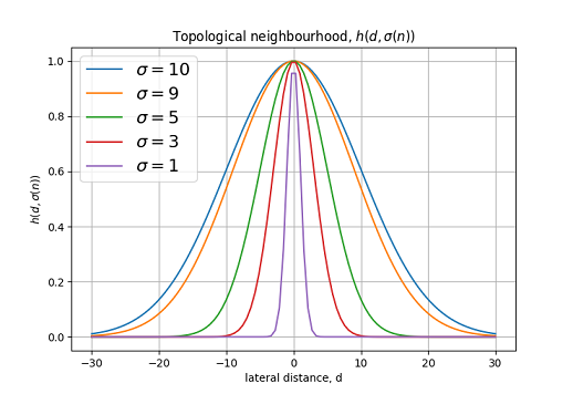
Graph of topological neighborhood function for various .
SOM is characterized by a decrease in the topological neighborhood in the learning process. You can achieve this by changing according to the formula:

Schedule change in the process of studying.
Function at the end of the training phase should cover only the nearest neighbors. The figures below show the graphs of the topological neighborhood function for a two-dimensional lattice.
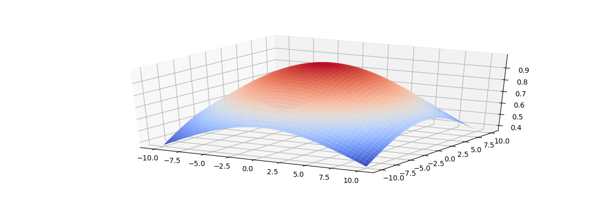
From this figure it is clear that at the beginning of the training, the topological neighborhood covers almost the entire lattice.

At the end of training tapers to nearest neighbors.
Step 5: Adaptation Process. The adaptation process involves changing the synaptic weights of the network. Changing the weight vector of the neuron in the lattice can be expressed as follows:
As a result, we have the formula of the updated weights vector at the moment of time :
The SOM learning algorithm also recommends changing the learning speed parameter. depending on the step.
Where Is another constant of the SOM algorithm.

Schedule change in the process of studying.
After updating the scales, we return to step 2, and so on.
Network training consists of two stages:
The stage of self-organization can take up to 1000 iterations and maybe more.
Convergence stage - required for fine-tuning the feature map. As a rule, the number of iterations sufficient for the convergence stage can exceed the number of neurons in the network by 500 times.
Heuristics 1. The initial value of the learning rate parameter is better to choose close to the value: , . However, it should not fall below the value of 0.01.
Heuristics 2. Original value should be set approximately equal to the lattice radius, and the constant stupid like:
Now let's move on from theory to practical implementation of a self-organizing map (SOM) using Python and TensorFlow.
To begin, create the SOMNetwork class and create TensorFlow operations to initialize all the constants:
Next, create a function to create the operation of the competition process:
It remains for us to create the main learning operation for the processes of cooperation and adaptation:
As a result, we implemented SOM and received the operation training_op with the help of which we can train our neural network, passing the input vector and step number as a parameter at each iteration. Below is a graph of TensorFlow operations built using Tesnorboard.
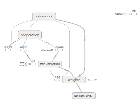
Graph operations TensorFlow.
To test the program, we will feed a three-dimensional vector to the input. . This vector can be represented as a color of three component.
Let's create an instance of our SOM network and an array of random vectors (colors):
Now you can implement the main learning cycle:
After learning, the network converts a continuous input color space into a discrete gradient map, when feeding a single color gamut, neurons will always be activated from one map area corresponding to a given color (one neuron is activated which is the most suitable to the supplied vector). For demonstration, one can imagine the vector of synaptic weights of neurons as a color gradient image.
The figure shows a scale map for a network of 20x20 neurons, after 200 thousand. learning iterations:
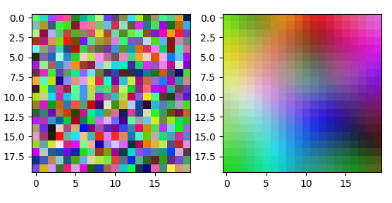
Map of weights at the beginning of training (left) and at the end of training (right).

Scale map for a network of 100x100 neurons, after 350 thousand. iterations of learning.
As a result, a self-organizing map was created and an example of its training on the input vector consisting of three components is shown. For learning the network, you can use a vector of any dimension. You can also convert the algorithm to work in batch mode. In this case, the order of presentation of the network of input data does not affect the final form of the attribute map and there is no need to change the learning speed parameter with time.
PS: The full program code can be found here .
About self-organization cards
To begin with, let's figure out what the Self-orginizing Map is, or simply SOM. SOM is an artificial neural network based on learning without a teacher. In self-organizing maps, neurons are placed in lattice sites, usually one- or two-dimensional. All neurons of this lattice are connected with all nodes of the input layer.
SOM transforms continuous source space to discrete output space .
SOM learning algorithm
Network training consists of three main processes: competition , cooperation and adaptation . The following describes all the steps of the SOM learning algorithm.
')
Step 1: Initialization. For all the vectors of synaptic weights,
Where - the total number of neurons, - dimension of the input space, selects a random value from -1 to 1.
Step 2: Sub-selection. Choose a vector from the input space.
Step 3: Search for a winning neuron or process competition. Find the most suitable (winning neuron) on the move , using the minimum Euclidean distance criterion (which is equivalent to the maximum of scalar products ):
Euclidean distance.
Euclidean distance ( ) are defined as:
Step 4: The process of cooperation. The winning neuron is located in the center of the topological neighborhood of the “cooperating” neurons. The key question is: how to define the so-called topological neighborhood (topological neighborhood) of the victorious neuron? For convenience, we denote it by the symbol: , centered on the victorious neuron . The topological neighborhood must be symmetric with respect to the maximum point determined when , - this is the lateral distance between the winner and neighboring neurons .
A typical example satisfying the condition above is the gauss function :
Where - effective width. Lateral distance is defined as: in one dimensional, and: in the two-dimensional case. Where determines the position of the excited neuron, and - position of the winning neuron (in the case of a two-dimensional lattice where and coordinates of the neuron in the lattice).
Graph of topological neighborhood function for various .
SOM is characterized by a decrease in the topological neighborhood in the learning process. You can achieve this by changing according to the formula:
Where - some constant - learning step - initial value .
Schedule change in the process of studying.
Function at the end of the training phase should cover only the nearest neighbors. The figures below show the graphs of the topological neighborhood function for a two-dimensional lattice.
From this figure it is clear that at the beginning of the training, the topological neighborhood covers almost the entire lattice.
At the end of training tapers to nearest neighbors.
Step 5: Adaptation Process. The adaptation process involves changing the synaptic weights of the network. Changing the weight vector of the neuron in the lattice can be expressed as follows:
- parameter learning speed.
As a result, we have the formula of the updated weights vector at the moment of time :
The SOM learning algorithm also recommends changing the learning speed parameter. depending on the step.
Where Is another constant of the SOM algorithm.
Schedule change in the process of studying.
After updating the scales, we return to step 2, and so on.
Heuristics SOM learning algorithm
Network training consists of two stages:
The stage of self-organization can take up to 1000 iterations and maybe more.
Convergence stage - required for fine-tuning the feature map. As a rule, the number of iterations sufficient for the convergence stage can exceed the number of neurons in the network by 500 times.
Heuristics 1. The initial value of the learning rate parameter is better to choose close to the value: , . However, it should not fall below the value of 0.01.
Heuristics 2. Original value should be set approximately equal to the lattice radius, and the constant stupid like:
At the stage of convergence, the change should be stopped. .
Implementing SOM with Python and TensorFlow
Now let's move on from theory to practical implementation of a self-organizing map (SOM) using Python and TensorFlow.
To begin, create the SOMNetwork class and create TensorFlow operations to initialize all the constants:
import numpy as np import tensorflow as tf class SOMNetwork(): def __init__(self, input_dim, dim=10, sigma=None, learning_rate=0.1, tay2=1000, dtype=tf.float32): # if not sigma: sigma = dim / 2 self.dtype = dtype # self.dim = tf.constant(dim, dtype=tf.int64) self.learning_rate = tf.constant(learning_rate, dtype=dtype, name='learning_rate') self.sigma = tf.constant(sigma, dtype=dtype, name='sigma') # 1 ( 6) self.tay1 = tf.constant(1000/np.log(sigma), dtype=dtype, name='tay1') # 1000 ( 3) self.minsigma = tf.constant(sigma * np.exp(-1000/(1000/np.log(sigma))), dtype=dtype, name='min_sigma') self.tay2 = tf.constant(tay2, dtype=dtype, name='tay2') #input vector self.x = tf.placeholder(shape=[input_dim], dtype=dtype, name='input') #iteration number self.n = tf.placeholder(dtype=dtype, name='iteration') # self.w = tf.Variable(tf.random_uniform([dim*dim, input_dim], minval=-1, maxval=1, dtype=dtype), dtype=dtype, name='weights') # , self.positions = tf.where(tf.fill([dim, dim], True)) Next, create a function to create the operation of the competition process:
def __competition(self, info=''): with tf.name_scope(info+'competition') as scope: # distance = tf.sqrt(tf.reduce_sum(tf.square(self.x - self.w), axis=1)) # ( 1) return tf.argmin(distance, axis=0) It remains for us to create the main learning operation for the processes of cooperation and adaptation:
def training_op(self): # win_index = self.__competition('train_') with tf.name_scope('cooperation') as scope: # d # 1d 2d coop_dist = tf.sqrt(tf.reduce_sum(tf.square(tf.cast(self.positions - [win_index//self.dim, win_index-win_index//self.dim*self.dim], dtype=self.dtype)), axis=1)) # ( 3) sigma = tf.cond(self.n > 1000, lambda: self.minsigma, lambda: self.sigma * tf.exp(-self.n/self.tay1)) # ( 2) tnh = tf.exp(-tf.square(coop_dist) / (2 * tf.square(sigma))) with tf.name_scope('adaptation') as scope: # ( 5) lr = self.learning_rate * tf.exp(-self.n/self.tay2) minlr = tf.constant(0.01, dtype=self.dtype, name='min_learning_rate') lr = tf.cond(lr <= minlr, lambda: minlr, lambda: lr) # ( 4) delta = tf.transpose(lr * tnh * tf.transpose(self.x - self.w)) training_op = tf.assign(self.w, self.w + delta) return training_op As a result, we implemented SOM and received the operation training_op with the help of which we can train our neural network, passing the input vector and step number as a parameter at each iteration. Below is a graph of TensorFlow operations built using Tesnorboard.
Graph operations TensorFlow.
Testing the program
To test the program, we will feed a three-dimensional vector to the input. . This vector can be represented as a color of three component.
Let's create an instance of our SOM network and an array of random vectors (colors):
# 2020 som = SOMNetwork(input_dim=3, dim=20, dtype=tf.float64, sigma=3) test_data = np.random.uniform(0, 1, (250000, 3)) Now you can implement the main learning cycle:
training_op = som.training_op() init = tf.global_variables_initializer() with tf.Session() as sess: init.run() for i, color_data in enumerate(test_data): if i % 1000 == 0: print('iter:', i) sess.run(training_op, feed_dict={som.x: color_data, som.n:i}) After learning, the network converts a continuous input color space into a discrete gradient map, when feeding a single color gamut, neurons will always be activated from one map area corresponding to a given color (one neuron is activated which is the most suitable to the supplied vector). For demonstration, one can imagine the vector of synaptic weights of neurons as a color gradient image.
The figure shows a scale map for a network of 20x20 neurons, after 200 thousand. learning iterations:
Map of weights at the beginning of training (left) and at the end of training (right).
Scale map for a network of 100x100 neurons, after 350 thousand. iterations of learning.
Conclusion
As a result, a self-organizing map was created and an example of its training on the input vector consisting of three components is shown. For learning the network, you can use a vector of any dimension. You can also convert the algorithm to work in batch mode. In this case, the order of presentation of the network of input data does not affect the final form of the attribute map and there is no need to change the learning speed parameter with time.
PS: The full program code can be found here .
Source: https://habr.com/ru/post/334810/
All Articles