Machine learning in skiing

This article will discuss the possibilities of using machine learning for the analysis of biomechanics in alpine skiing.



Initially, the hypothesis of these possibilities has been reduced to the following set of requirements:

')

• ability to classify technical elements;
• ability to compare specified elements according to a certain metric; find non-trivial features of the route, to minimize the time;
• ability to make predictions (for example, for a second attempt).

For the initial testing of this hypothesis, we decided to train an artificial neural network (hereinafter ANN) to recognize the simplest phases of the trajectory of an athlete-mountain skier.



The stages of work are defined as follows:



1. Data collection.

2. Preparation of data for training.

3. Training the network to recognize whole turns.

4. Network training on the recognition of the phases of turns.

5. Development of a service for users to work with the resulting system.

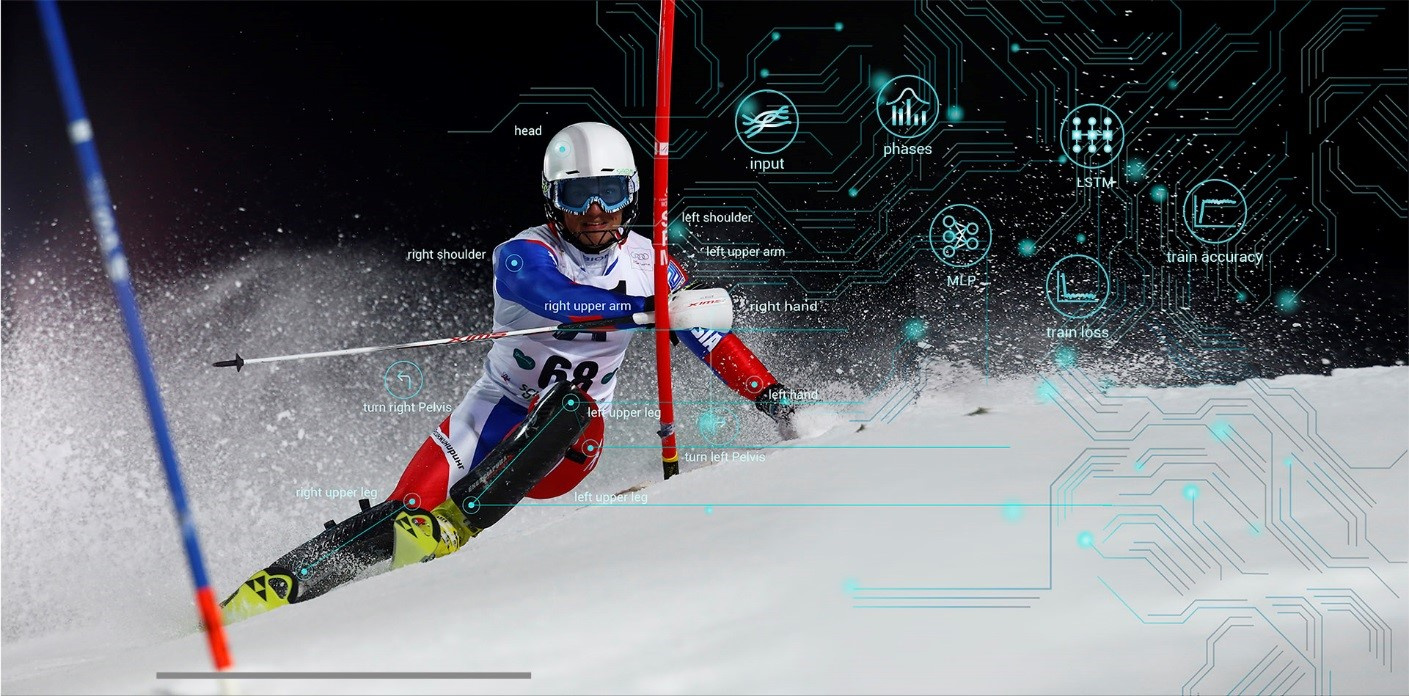
Data collection. Motion capture

What data to collect? How to get them?



There are quite a lot of indicators that characterize the athlete's activity during the descent, ranging from the pressure profile of the foot to the ski boot (it is from these inconspicuous movements that all movement control begins) and ending with the direction of gaze (than at the gate farther from the athlete he looks, the higher the chance of building the optimal trajectory). To begin with, we decided to dwell exclusively on motion capture (MoCap), that is, to obtain a skeletal model of the movement of body segments, since this approach most widely describes the physics of the process.



Motion capture was done using Xsens solution (MVN Biomech),

which is a nylon jumpsuit with installed inertial sensors (IMU). According to its characteristics, the suit remotely resembles the standard sports equipment - “trigger suit”, which allows the athlete, with some limitations, to simply wear it under the usual equipment.



In operation, we had to adapt the original solution for authentic ski equipment. This was done primarily to improve the accuracy of data recording (some sensors were poorly attached), and the second to speed up the process of preparing for skating. As a result, the athlete, when wearing a uniform or driving, will hardly feel the difference between recording biomechanics and regular training.

Data preparation

Before we talk about the preparation of raw data, we should explain what we understand by them.



The MoCap system records motion in frames, in simple terms frames, in each of which we have a description of the body position in 23 segments, each of which, in turn, is defined by its quaternion (an object of linear algebra with which solid-state rotations are described; it is analogous to Euler angles , but easier in terms of operations). Each quaternion describes the rotation of a body segment relative to its original position in global space. Frames are written with a frequency of 240Hz, which allows you to catch quite fast movements, for example, beating the brush at the time of the injection with a stick.



Now, directly, as for preparation.



For a start, we take and leave only the driveways themselves, throwing out everything that happens between (rises on the yoke, waiting, etc.). As a result - out of ten workouts suitable for work (there were a lot of defects due to the installation of sensors and their subsequent displacement), there were five. On average, each training session recorded twenty passages, the useful time of each of which is thirty seconds. Total we get 5 trainings * 20 passages * 30 seconds * 240 Hz = 720 000 frames; well, or if we go further 720,000 frames * 23 segments * 4 real numbers in quaternion = about 66 million real numbers. It sounds like it is enough.



Next, you need to manually mark the data for training - to explain to the neural network what exactly it should recognize. And the goal was to teach her to recognize first full turns, and then their phases. For this, visualization of movements and indicators of key segments (in our case, feet, tibia) were viewed and on the timeline marks of the beginning and end of the corresponding elements were placed. Thus, on the basis of all the records, we got about 3,500 turns, or 10,500 phases.



The last thing that had to be done in preparation was to bring the turn angles of the segments from global to local angles of the joints of the segments. The biomechanical model has a clear hierarchy of articulations of segments, along which the whole construction proceeds from raw data. It was necessary for each segment, except the root, to obtain the quaternion of the angle of the joint for this element. The root segment in this hierarchy is the pelvis. Obviously, knowing the turns of the segments and their lengths along the chain (and this data is there, since an anthropometric profile is recorded for each athlete), the entire biomechanical model can be restored. It remained to perform normalization of the pelvic in azimuth in the global space, and data were obtained that did not depend on the orientation of the athlete in space.

Data quality

The analysis of the quality of primary data was carried out using Python packages: Jupyter, NumPy, MatPlotLib and TensorFlow.



Here it is worthwhile to dwell on two essential points.



The first - the data from some segments were "noise" - they changed either randomly or not at all. There were also segments that gave adequate data, but were substantially similar in the whole range of movements, which practically meant their linear dependence. For example, two adjacent spinal segments could have the same behavior, so there was no point in using both.



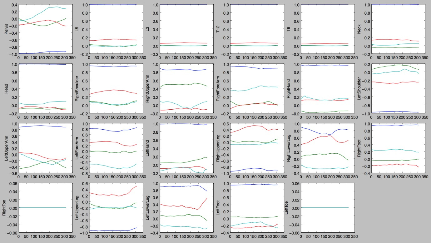
1. Graphs of changes in the quaternions of the angles of the joints of the segments when performing a right turn



The illustration clearly shows that not all the values ​​of the segments quite clearly demonstrate the nature of the action and are useful for learning. They can be useful for analyzing the quality of an action and its characteristics, but not for automatic marking of actions.



The second significant moment is the sign instability of the quaternion components. What it is? The same turn in their language can be described by two different sets of four numbers. For example, the same rotation around the X axis by 180 and around the Y axis by 90 can be equally represented by the following quaternions: (0.0.7,0,0.7) and (0, -0.7.0, -0.7).





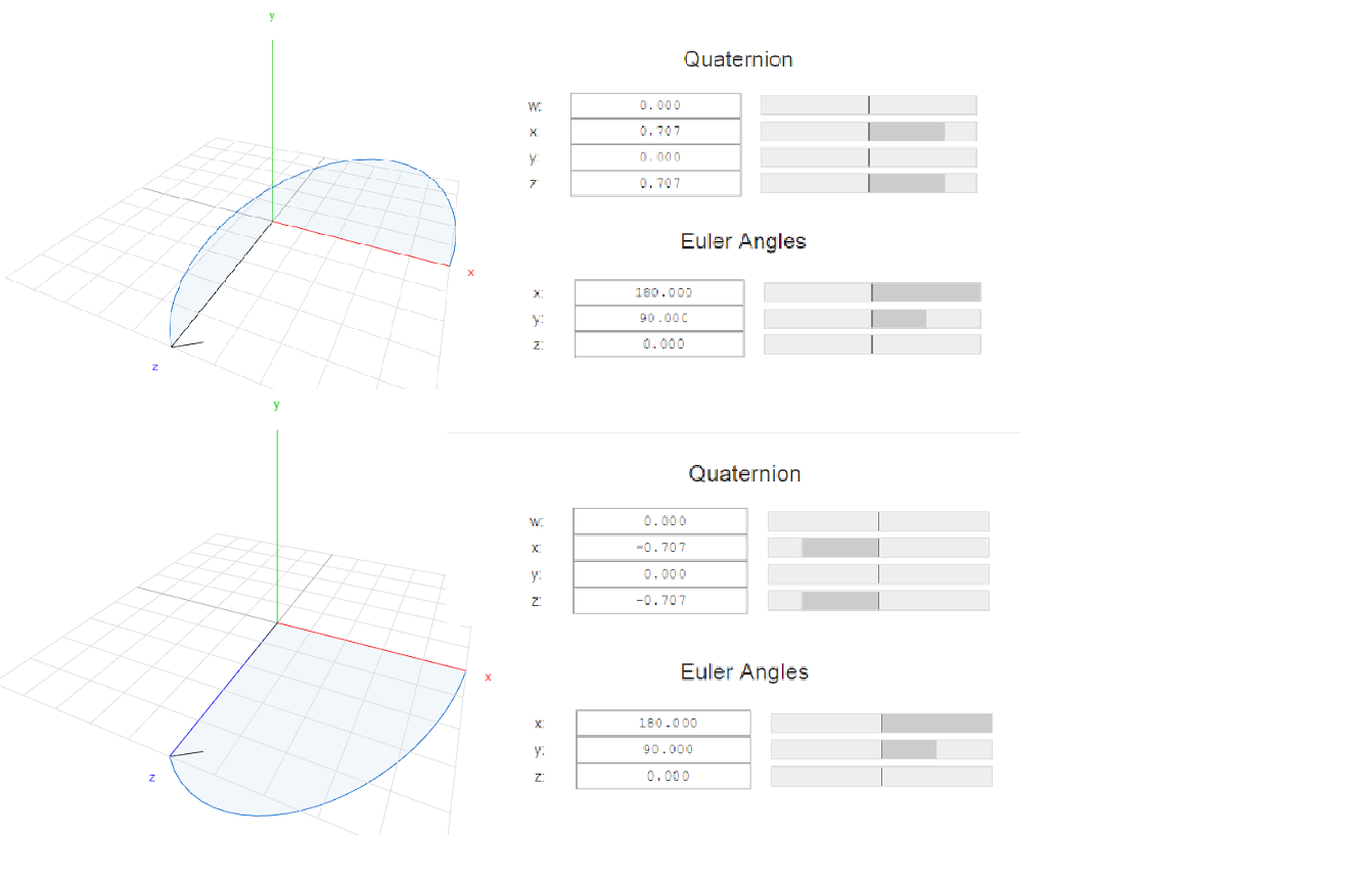
2. Different representation of rotation by quaternions



Why is it important? The fact is that without separate data arrays for different paths, the same turns can have a sign inversion for individual components. Looking ahead, we note that the neural network will initially perceive them as different situations. And in space and time, this inversion occurs absolutely spontaneously.





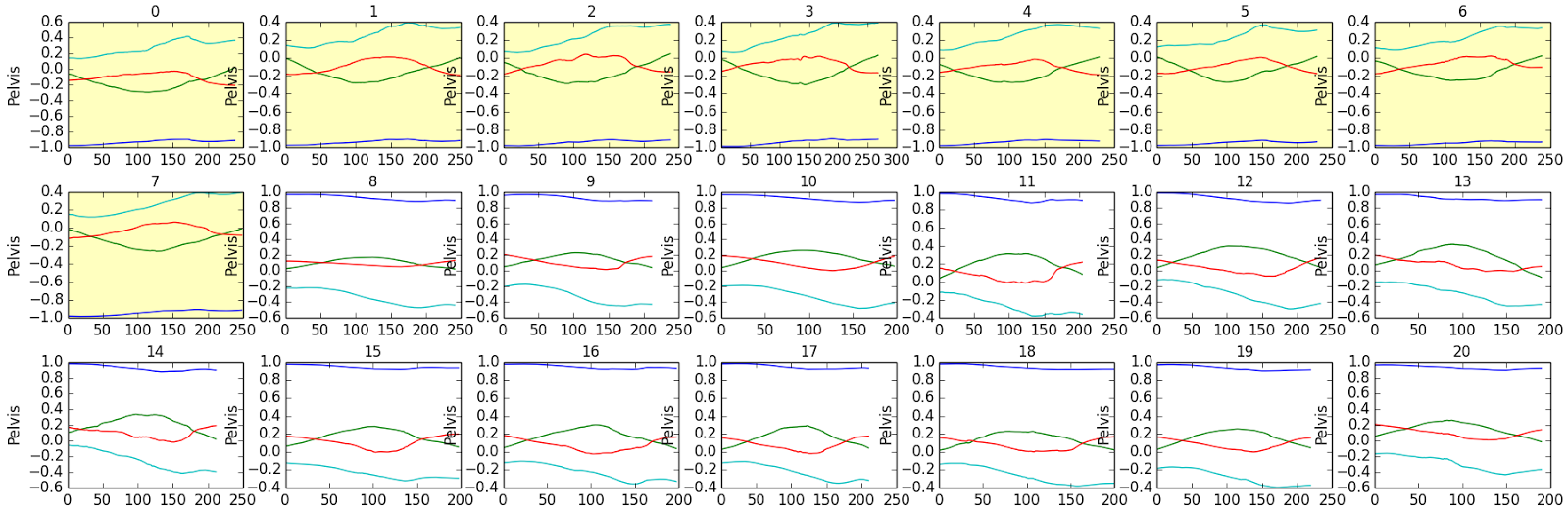
3. An example of sign input instability



For one of the races in this figure, the graphs of changing the quaternion of the athlete's pelvis in the right turn are highlighted in yellow, for the other - in white. Values ​​are equivalent and display the same angles, but due to the properties of quaternions they may have opposite signs of the components. How we managed to cope with this feature is described below.

Network training on the definition of whole turns

A bit of materiel on ski discipline: recorded data slalom turns (slalom - the least speed of the ski disciplines, which is characterized by turns of small radius, closely spaced gates and, as a consequence, a large frequency of turns), the average duration of which ranged from 0.9 to + - 0.1 seconds . To begin with, it was very opportune that the slowest and fastest turns in our data differed less than twice in duration.



To create a prototype of the recognition system for whole turns, using the TensorFlow package, we created and trained an MLP network (multilayer perceptron) with two hidden layers of 256 neurons (the network graph is shown in Figure 3). Data sampling for training and rotation recognition was performed using the sliding window method with a size exceeding the longest known duration of the whole rotation. The network was trained to recognize that the entire turn was hitting the data window. Sliding the window recognized the start and end of the turn.





4. Count the trained MLP network with two hidden layers of 256 neurons.



It is worth a little bit to dwell on how at this stage we solved the data preparation problems described above. For this rather trivial task, the approach to the problems of “noisy segments” and the sign instability of quaternions was the same - we simply throw them out. Data volumes were enough to simply not train the network, not only on noisy segments, but also on data where the quaternions were inverted.



The approach worked, but later I had to return to this task more carefully. Without special actions, the network sees the difference between the components of the quaternion and perceives them as different objects, without generalizing them. In order for her to learn to notice the similarities in quaternions with different component signs, she had to be trained in a special way - but at the next stage, about which below.



As can be seen in Figure 5, the network showed good learning.





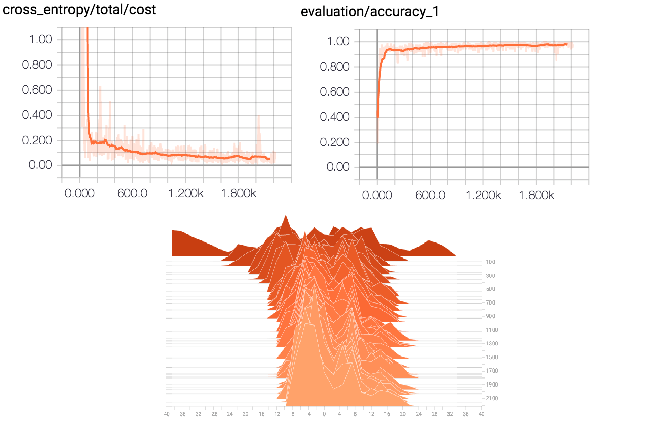
5. Network learning.



As a result, at this stage, we confirmed the possibility of determining whole turns, also clarified the criteria for data preparation.

We train the network on phases of turns

Now it is time to move to the phases of turns. And again, a little materiel.



In the simplest case, there are three phases:



1. Entrance to a turn (characterized by a rapid increase in the edge angle of the skis and generally high first and second derivatives in almost all relative positions of the segments. Simply put, the skier very quickly changes from a relatively straight position to the state “turned into a turn”: the knees are bent, the pelvis strongly pronounced in the direction of rotation, pronounced raznozhka). The average length is 0.25 seconds.



2. Hold in turn (the phase in which the skier holds the body position formed in the first phase, naturally with some fluctuations. That is, we first prepared and now perform the main arc. This corresponds to the gap between the flags. In terms of biomechanical indicators, it looks like fluctuations around zero marks of relative accelerations and speeds). The average length is 0.4 seconds.



3. Getting out of the turn (This phase of the mirror is first, it is rapidly returning from the “deeply pledged” to the direct state, as well as the first phase we see an explosive growth of relative velocities and accelerations, naturally with opposite data). The average length is 0.25 seconds.



It is important to clarify that all the above-described division into phases is highly contextual and highly dependent on the placement of flags, coverage, and so on. Sometimes in the retention phase, atypical activity may occur. Even more complicated is the transition from one phase to another, since in reality there is no abrupt stopping of some indicator, but there is a certain threshold level of attenuation on a whole group of segments, which can be used to conclude about the change of phases. And all this was to teach our network.





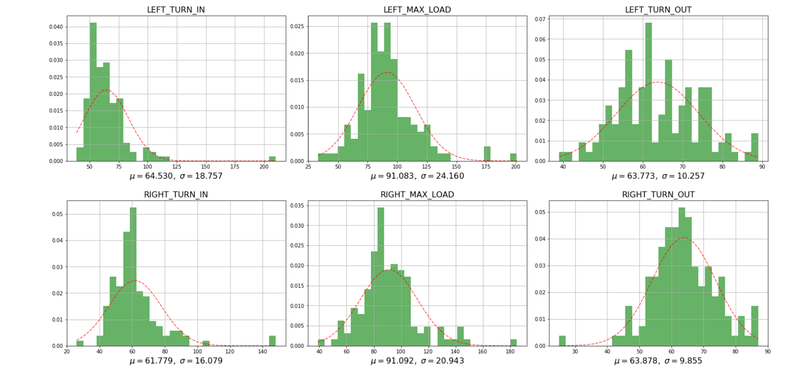
6. Estimation of the phase length variation.



Looking at the statistics of the phases can be seen as their significant differences in the average length, and significantly greater variance compared to whole turns, and as a result we could not find a window of this size for learning that any turn would fall into, but two consecutive . This forced to abandon the sliding window method.



Accordingly, it was decided to move from the MLP network to the RNN / LSTM network.





7. Graph "trained" RNN / LSTM-network



But this is half the trouble. Even more “interesting” things were with sign instability. If in the case of whole turns it was possible to just throw out inverted segments, then they decided to act smarter. Namely, the stochastic method.



When loading the original data sets, artificial data sets were created, repeating the data of the original, but having a sign inversion of the quaternion parameters in a randomly selected segment, which were “fed” by the network, training it with artificial anomalies. The volume of data has grown, and the INS has learned to understand that the data can sometimes lie, but they also say the same thing. As a result, she learned to recognize the phases of movements regardless of the sign of the quaternion components.



And then - the matter of technology, and as a result a qualitatively trained network was obtained, that is, giving good recognition accuracy on new data. Below is its graph and phase recognition results.







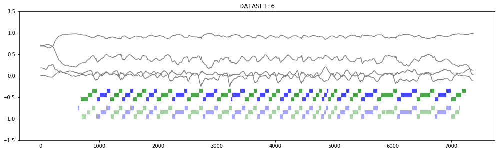
8. Phase recognition result in race №6. Steps show the known types of phases: entry, maximum load and turn out. Saturated colors marked control markup, pale - the results of recognition. Green turns left turns, blue - right. The recognition result was not subjected to additional filtering or post-processing.



Summing up, we can say that as a result, a neural network receiving an entry for a skier on a slalom track makes phase marking, creating labels on the time scale of the beginning and end of each phase.

User interface

In order to give the solution a custom look, we decided to create a service that allows us to do the following:



1. Send a biomechanical record of a slalom passage to the service, including as a stream of real-time data

2. Get markup in response (annotated entry)

3. View the ride in the render of a skier with visualization of phase markings.



Below is a diagram of the service:



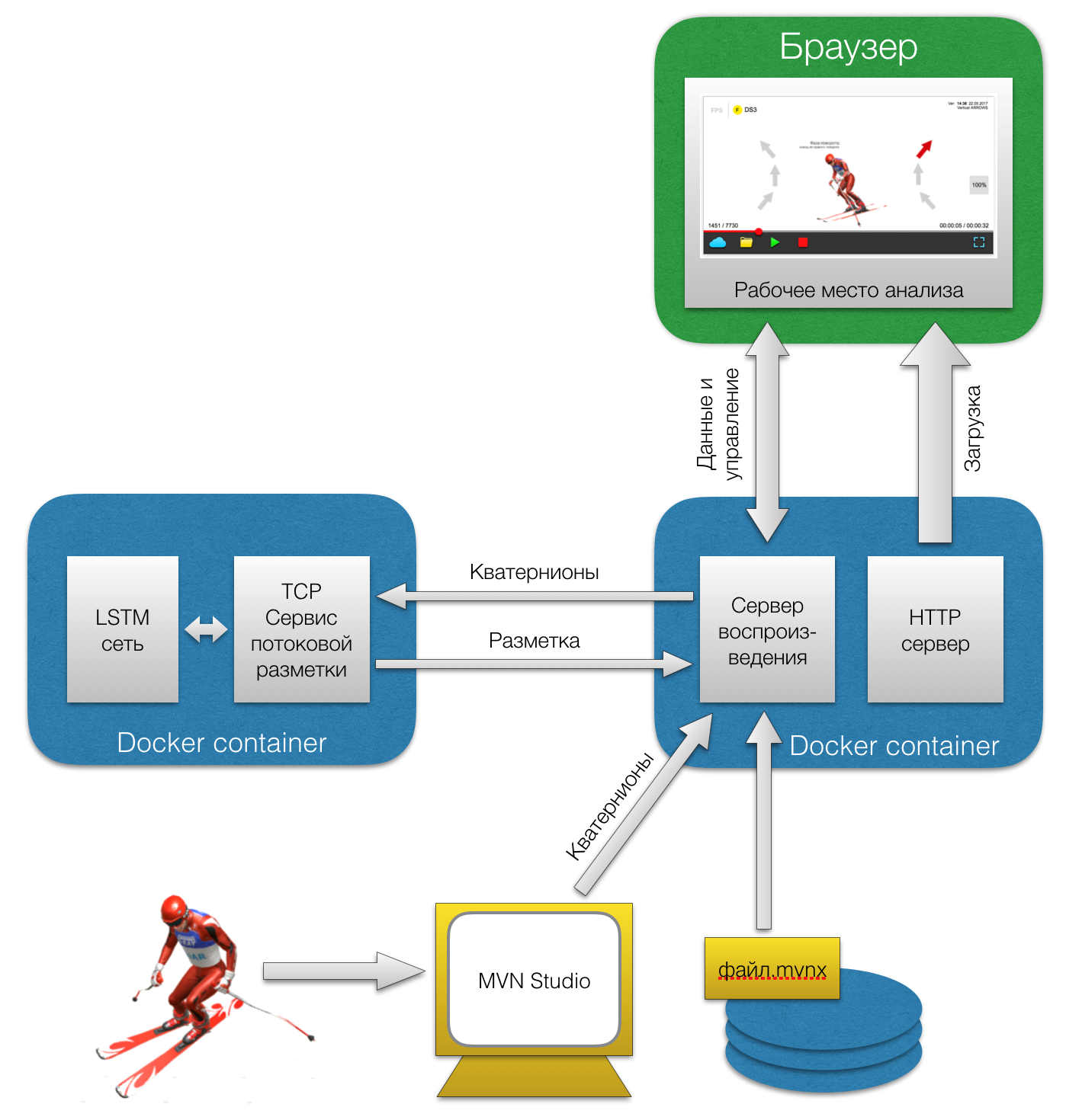
9. System Services for Stream Phase Marking



Its main components are the RNN / LSTM network, a network streaming markup service, a playback server, and a phase analysis workstation made in the form of a web application.



In this form, this service is more likely a demonstration of possibilities than an instrument that solves applied problems, but it is a necessary liner to our big task. Looking ahead, we can say that the markup is necessary for the subsequent analysis of comparable technical fragments.

What's next?

The goal of the current year is a system capable of classifying and evaluating, starting with the behavior of an individual body segment in the context of the phase (possibly more detailed than in the description above), and further with increasing degree of generalization: rotation, link, track, level of skiing in general. Most importantly, we are planning to build on all the above elements of the quality metric.

Conclusion

Separately, I would like to say that a region of significant shortage of raw data was found, namely, describing the human locomotion, or, more simply, data on how we move. The presence of such would allow to radically expand the field of application of machine learning, as it once happened with visual images.



In this regard, we want to invite experts, and just people who are interested in this area, to cooperate. The format of this cooperation is left open.



We are waiting for your feedback!