Traffic Sign Recognition with CNN: Image Preprocessing Tools
Hi, Habr! Continuing a series of materials from a graduate of our program Deep Learning , Cyril Danilyuk, on the use of convolutional neural networks for pattern recognition - CNN (Convolutional Neural Networks)
Over the past few years, the field of computer vision (CV) is experiencing, if not a rebirth, then a huge surge of interest in itself. In many ways, this increase in popularity is associated with the evolution of neural network technologies. For example, convolutional neural networks (convolutional neural networks or CNN) have selected a large chunk of tasks for generating features previously solved by the classical CV: HOG, SIFT, RANSAC, etc. methods.
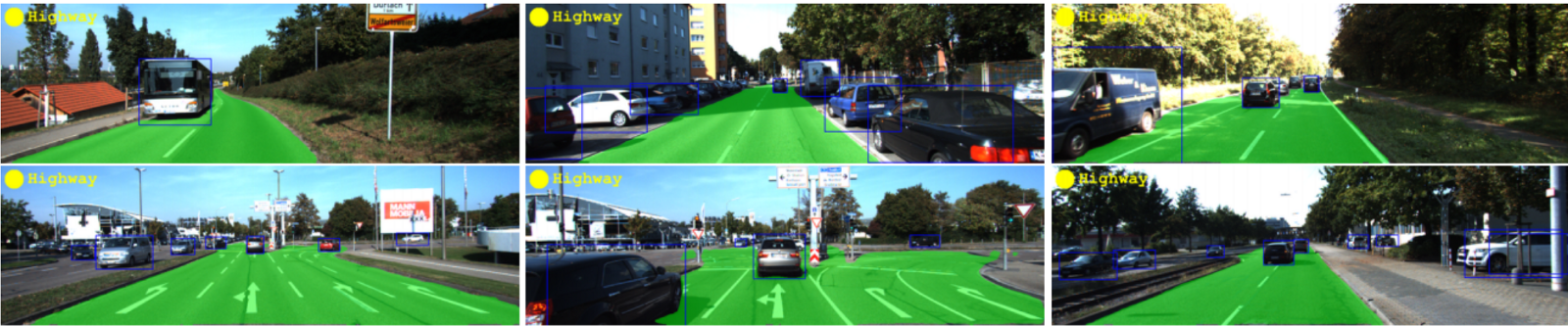
Mapping, image classification, building a route for drones and unmanned vehicles - many tasks related to feature generation, classification, image segmentation can be effectively solved using convolutional neural networks.
')
MultiNet as an example of a neural network (three in one), which we will use in one of the following posts. A source.
It is assumed that the reader has a general understanding of the work of neural networks. The network has a huge number of posts, courses and books on this topic. For example:
Tip: To make sure that you know the basics of neural networks, write your network from scratch and play with it!
Instead of repeating the basics, this series of articles focuses on several specific neural network architectures: STN (spatial transformer network), IDSIA (convolutional neural network for the classification of road signs), NVIDIA's neural network for end-to-end autopilot development and MultiNet for recognition and the classification of road markings and signs. Let's get started!
The topic of this article is to show several tools for image preprocessing. The overall pipeline usually depends on a specific task, but I would like to dwell on the tools. Neural networks are not the same magical black boxes that they like to present in the media: you can not just take and “throw” the data into the grid and wait for the magical results. By the rule of shit in - shit out at best, you will get a score worse by a few points. And, most likely, you just won't be able to train the network and no fancy techniques like normalization of batch or dropout will help you. Thus, the work must begin with the data: their cleaning, normalization and normalization. Additionally, it is worth thinking about expanding (data augmentation) of the original image dataset using affine transformations such as rotation, shifts, changing the scale of pictures: this will help reduce the likelihood of retraining and ensure better class invariance to transformations.
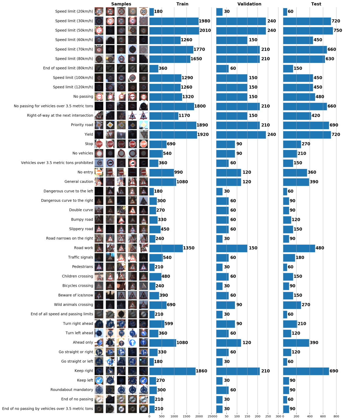
Within this and the next posts we will use GTSRB - dataset for the recognition of road signs in Germany. Our task is to train a road sign classifier using tagged data from GTSRB. In general, the best way to get an idea of the available data is to build a histogram of the distribution of the train, validation and / or test data sets:
Basic information about our dataset:
At this stage,
As a result, just one graph can tell a lot about our data set. Below are 3 tasks that can be solved using a well-constructed schedule:
In order to improve the convergence of the neural network, it is necessary to bring all the images to a single illumination by (as recommended in the LeCun article on the recognition of road signs) converting their color gamut into grayscale. This can be done both with the help of OpenCV, and with the help of the excellent Python library
I note that
Our approach to parallelization is very simple: we divide the sample into batchy and process each batch independently of the others. Once all the batch files are processed, we merge them back into one data set. My implementation of CLAHE is shown below:
Now that the transformation itself is ready, we will write a code that applies it to each batch from the training set:
Finally, apply the written function to the training set:
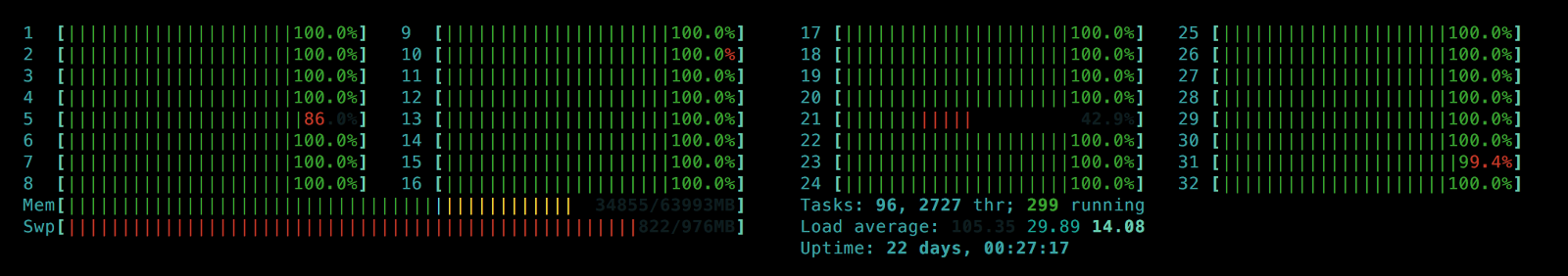
As a result, we use not one, but all the processor cores (32 in my case) and get a significant increase in performance. Sample received images:
The result of the normalization of images and the transfer of their color range in grayscale
Normalization of distribution for RGB images (I used another function for rc [:]. Map)
Now the whole process of data preprocessing takes several tens of seconds, so we can test different values of the number of intervals

num_bins: 8, 32, 128, 256, 512
Choosing a larger number of
Finally, use ipython magic
It is not a secret to anyone that adding new diverse data to a sample reduces the likelihood of retraining a neural network. In our case, we can construct artificial images by transforming the existing images with the help of rotation, specular reflection and affine transformations. Despite the fact that we can conduct this process for the entire sample, save the results and then use them, the more elegant way will be to create new images on the fly (online) so that you can quickly adjust the data augmentation parameters.
To begin with, we denote all the planned transformations using
Scaling and
Part of the conversion table. The values in the cells indicate the class number that will receive this image after transformation. Empty cells mean that this conversion is not available for this class.
Note that the column headings correspond to the names of the transforming functions defined earlier, so that during processing you can add transformations:
Now we can build a pipeline that applies all the available functions (transformations) listed in
Fine! Now we have 2 ready data augmentation functions:
The final step is to create a batch generator:
Combining datasets with different numbers of
Generated with augmented_batch_generator images
Note: augmentation is needed for train set. We also process the test set, but do not augment it.
Let's check that we inadvertently did not violate the distribution of classes on the extended train compared to the original dataset:
Left: histogram of data distribution from augmented batch generator. Right: the original train. As you can see, the values are different, but the distributions are similar.
After the data preprocessing is completed, all the generators are ready and the data is ready for analysis, we can proceed to the training. We will use a double convolutional neural network: the STN (spatial transformer network) accepts pre-processed batchy of images from the generator and focuses on the road signs, while the IDSIA neural network recognizes the road sign on the images received from the STN. The next post will be devoted to these neural networks, their training, quality analysis and demo version of their work. Follow new posts!
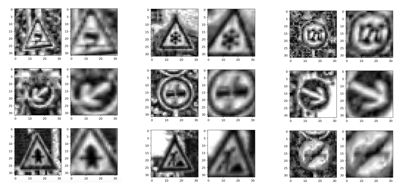
Left: The original pre-processed image. Right: a transformed STN image that takes as input the IDSIA for classification.
Introduction
Over the past few years, the field of computer vision (CV) is experiencing, if not a rebirth, then a huge surge of interest in itself. In many ways, this increase in popularity is associated with the evolution of neural network technologies. For example, convolutional neural networks (convolutional neural networks or CNN) have selected a large chunk of tasks for generating features previously solved by the classical CV: HOG, SIFT, RANSAC, etc. methods.
Mapping, image classification, building a route for drones and unmanned vehicles - many tasks related to feature generation, classification, image segmentation can be effectively solved using convolutional neural networks.
')
MultiNet as an example of a neural network (three in one), which we will use in one of the following posts. A source.
It is assumed that the reader has a general understanding of the work of neural networks. The network has a huge number of posts, courses and books on this topic. For example:
- Chapter 6: Deep Feedforward Networks - a chapter from the book Deep Learning by I.Goodfellow, Y.Bengio and A.Courville. Highly recommend.
- CS231n Convolutional Neural Networks for Visual Recognition is a popular course from Fei-Fei Li and Andrej Karpathy from Stanford. The course contains excellent materials focusing on practice and design.
- Deep Learning - course from Nando de Freitas from Oxford.
- Intro to Machine Learning - a free course from Udacity for beginners with an accessible presentation of the material, affects a large number of topics in machine learning.
Tip: To make sure that you know the basics of neural networks, write your network from scratch and play with it!
Instead of repeating the basics, this series of articles focuses on several specific neural network architectures: STN (spatial transformer network), IDSIA (convolutional neural network for the classification of road signs), NVIDIA's neural network for end-to-end autopilot development and MultiNet for recognition and the classification of road markings and signs. Let's get started!
The topic of this article is to show several tools for image preprocessing. The overall pipeline usually depends on a specific task, but I would like to dwell on the tools. Neural networks are not the same magical black boxes that they like to present in the media: you can not just take and “throw” the data into the grid and wait for the magical results. By the rule of shit in - shit out at best, you will get a score worse by a few points. And, most likely, you just won't be able to train the network and no fancy techniques like normalization of batch or dropout will help you. Thus, the work must begin with the data: their cleaning, normalization and normalization. Additionally, it is worth thinking about expanding (data augmentation) of the original image dataset using affine transformations such as rotation, shifts, changing the scale of pictures: this will help reduce the likelihood of retraining and ensure better class invariance to transformations.
Tool 1: Visualization and Exploration Data Analysis
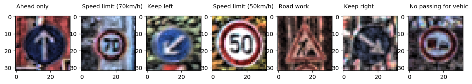
Within this and the next posts we will use GTSRB - dataset for the recognition of road signs in Germany. Our task is to train a road sign classifier using tagged data from GTSRB. In general, the best way to get an idea of the available data is to build a histogram of the distribution of the train, validation and / or test data sets:
Basic information about our dataset:
Number of training examples = 34799 Number of validation examples = 4410 Number of testing examples = 12630 Image data shape = (32, 32, 3) Number of classes = 43 At this stage,
matplotlib is your best friend. Despite the fact that using only pyplot you can perfectly visualize the data, matplotlib.gridspec allows matplotlib.gridspec to merge 3 graphics together: gs = gridspec.GridSpec(1, 3, wspace=0.25, hspace=0.1) fig = plt.figure(figsize=(12,2)) ax1, ax2, ax3 = [plt.subplot(gs[:, i]) for i in range(3)] Gridspec very flexible. For example, for each histogram you can set its width, as I did above. Gridspec considers the axis of each histogram independently of the others, which allows you to create complicated graphs.As a result, just one graph can tell a lot about our data set. Below are 3 tasks that can be solved using a well-constructed schedule:
- Image visualization. The graphics immediately show a lot of too dark or too light images, so a sort of data normalization must be done to eliminate the brightness variation.
- Check the sample for imbalance. If instances of a class prevail in the sample, it is necessary to use undersampling or oversampling methods.
- Check that the train, validation, and test sample distributions are similar. This can be checked by looking at the histograms above, or using the Spearman rank correlation coefficient. (via
scipy)
Tool 2: IPython Parallel for scikit-image
In order to improve the convergence of the neural network, it is necessary to bring all the images to a single illumination by (as recommended in the LeCun article on the recognition of road signs) converting their color gamut into grayscale. This can be done both with the help of OpenCV, and with the help of the excellent Python library
scikit-image , which can be easily installed with the help of pip (OpenCV also requires self-compilation with a bunch of dependencies). Image contrast normalization will be performed using adaptive histogram normalization (CLAHE, contrast limited adaptive histogram equalization):skimage.exposure.equalize_adapthist .I note that
skimage processes images one after another, using only one processor core, which is obviously inefficient. To parallelize image preprocessing, use the IPython Parallel library ( ipyparallel ). One of the advantages of this library is its simplicity: you can implement parallelized CLAHE with just a few lines of code. First, in the console (with ipyparallel installed), start the local ipyparallel cluster: $ ipcluster start Our approach to parallelization is very simple: we divide the sample into batchy and process each batch independently of the others. Once all the batch files are processed, we merge them back into one data set. My implementation of CLAHE is shown below:
from skimage import exposure def grayscale_exposure_equalize(batch_x_y): """Processes a batch with images by grayscaling, normalization and histogram equalization. Args: batch_x_y: a single batch of data containing a numpy array of images and a list of corresponding labels. Returns: Numpy array of processed images and a list of labels (unchanged). """ x_sub, y_sub = batch_x_y[0], batch_x_y[1] x_processed_sub = numpy.zeros(x_sub.shape[:-1]) for x in range(len(x_sub)): # Grayscale img_gray = numpy.dot(x_sub[x][...,:3], [0.299, 0.587, 0.114]) # Normalization img_gray_norm = img_gray / (img_gray.max() + 1) # CLAHE. num_bins will be initialized in ipyparallel client img_gray_norm = exposure.equalize_adapthist(img_gray_norm, nbins=num_bins) x_processed_sub[x,...] = img_gray_norm return (x_processed_sub, y_sub) Now that the transformation itself is ready, we will write a code that applies it to each batch from the training set:
import multiprocessing import ipyparallel as ipp import numpy as np def preprocess_equalize(X, y, bins=256, cpu=multiprocessing.cpu_count()): """ A simplified version of a function which manages multiprocessing logic. This function always grayscales input images, though it can be generalized to apply any arbitrary function to batches. Args: X: numpy array of all images in dataset. y: a list of corresponding labels. bins: the amount of bins to be used in histogram equalization. cpu: the number of cpu cores to use. Default: use all. Returns: Numpy array of processed images and a list of labels. """ rc = ipp.Client() # Use a DirectView object to broadcast imports to all engines with rc[:].sync_imports(): import numpy from skimage import exposure, transform, color # Use a DirectView object to set up the amount of bins on all engines rc[:]['num_bins'] = bins X_processed = np.zeros(X.shape[:-1]) y_processed = np.zeros(y.shape) # Number of batches is equal to cpu count batches_x = np.array_split(X, cpu) batches_y = np.array_split(y, cpu) batches_x_y = zip(batches_x, batches_y) # Applying our function of choice to each batch with a DirectView method preprocessed_subs = rc[:].map(grayscale_exposure_equalize, batches_x_y).get_dict() # Combining the output batches into a single dataset cnt = 0 for _,v in preprocessed_subs.items(): x_, y_ = v[0], v[1] X_processed[cnt:cnt+len(x_)] = x_ y_processed[cnt:cnt+len(y_)] = y_ cnt += len(x_) return X_processed.reshape(X_processed.shape + (1,)), y_processed Finally, apply the written function to the training set:
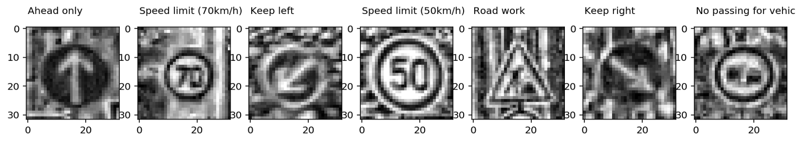
# X_train: numpy array of (34799, 32, 32, 3) shape # y_train: a list of (34799,) shape X_tr, y_tr = preprocess_equalize(X_train, y_train, bins=128) As a result, we use not one, but all the processor cores (32 in my case) and get a significant increase in performance. Sample received images:
The result of the normalization of images and the transfer of their color range in grayscale
Normalization of distribution for RGB images (I used another function for rc [:]. Map)
Now the whole process of data preprocessing takes several tens of seconds, so we can test different values of the number of intervals
num_bins in order to visualize them and select the most suitable:num_bins: 8, 32, 128, 256, 512
Choosing a larger number of
num_bins increases the contrast of the images, while at the same time highlighting their background, which makes the data noisy. Different values of num_bins can also be used to augment the dataset contrast by contrast so that the neural network does not retrain due to the background of the images.Finally, use ipython magic
%store to save the results for future reference: # Same images, multiple bins (contrast augmentation) %store X_tr_8 %store y_tr_8 # ... %store X_tr_512 %store y_tr_512 Tool 3: Online data augmentation
It is not a secret to anyone that adding new diverse data to a sample reduces the likelihood of retraining a neural network. In our case, we can construct artificial images by transforming the existing images with the help of rotation, specular reflection and affine transformations. Despite the fact that we can conduct this process for the entire sample, save the results and then use them, the more elegant way will be to create new images on the fly (online) so that you can quickly adjust the data augmentation parameters.
To begin with, we denote all the planned transformations using
numpy and skimage : import numpy as np from skimage import transform from skimage.transform import warp, AffineTransform def rotate_90_deg(X): X_aug = np.zeros_like(X) for i,img in enumerate(X): X_aug[i] = transform.rotate(img, 270.0) return X_aug def rotate_180_deg(X): X_aug = np.zeros_like(X) for i,img in enumerate(X): X_aug[i] = transform.rotate(img, 180.0) return X_aug def rotate_270_deg(X): X_aug = np.zeros_like(X) for i,img in enumerate(X): X_aug[i] = transform.rotate(img, 90.0) return X_aug def rotate_up_to_20_deg(X): X_aug = np.zeros_like(X) delta = 20. for i,img in enumerate(X): X_aug[i] = transform.rotate(img, random.uniform(-delta, delta), mode='edge') return X_aug def flip_vert(X): X_aug = deepcopy(X) return X_aug[:, :, ::-1, :] def flip_horiz(X): X_aug = deepcopy(X) return X_aug[:, ::-1, :, :] def affine_transform(X, shear_angle=0.0, scale_margins=[0.8, 1.5], p=1.0): """This function allows applying shear and scale transformations with the specified magnitude and probability p. Args: X: numpy array of images. shear_angle: maximum shear angle in counter-clockwise direction as radians. scale_margins: minimum and maximum margins to be used in scaling. p: a fraction of images to be augmented. """ X_aug = deepcopy(X) shear = shear_angle * np.random.rand() for i in np.random.choice(len(X_aug), int(len(X_aug) * p), replace=False): _scale = random.uniform(scale_margins[0], scale_margins[1]) X_aug[i] = warp(X_aug[i], AffineTransform(scale=(_scale, _scale), shear=shear), mode='edge') return X_aug Scaling and
rotate_up_to_20_deg turns rotate_up_to_20_deg increase the size of the sample, while maintaining the images belonging to the original classes. Reflections (flips) and rotations by 90, 180, 270 degrees can, on the contrary, change the meaning of the sign. To track such transitions, we will create a list of possible transformations for each road sign and the classes into which they will be converted (below is an example of a part of such a list):| label_class | label_name | rotate_90_deg | rotate_180_deg | rotate_270_deg | flip_horiz | flip_vert |
|---|---|---|---|---|---|---|
| 13 | Yield | 13 | ||||
| 14 | Stop | |||||
| 15 | No vehicles | 15 | 15 | 15 | 15 | 15 |
| sixteen | Vehicles over 3.5 ton prohibited | |||||
| 17 | No entry | 17 | 17 | 17 |
Note that the column headings correspond to the names of the transforming functions defined earlier, so that during processing you can add transformations:
import pandas as pd # Generate an augmented dataset using a transform table augmentation_table = pd.read_csv('augmentation_table.csv', index_col='label_class') augmentation_table.drop('label_name', axis=1, inplace=True) augmentation_table.dropna(axis=0, how='all', inplace=True) # Collect all global functions in global namespace namespace = __import__(__name__) def apply_augmentation(X, how=None): """Apply an augmentation function specified in `how` (string) to a numpy array X. Args: X: numpy array with images. how: a string with a function name to be applied to X, should return the same-shaped numpy array as in X. Returns: Augmented X dataset. """ assert augmentation_table.get(how) is not None augmentator = getattr(namespace, how) return augmentator(X) Now we can build a pipeline that applies all the available functions (transformations) listed in
augmentation_table.csv to all classes: import numpy as np def flips_rotations_augmentation(X, y): """A pipeline for applying augmentation functions listed in `augmentation_table` to a numpy array with images X. """ # Initializing empty arrays to accumulate intermediate results of augmentation X_out, y_out = np.empty([0] + list(X.shape[1:]), dtype=np.float32), np.empty([0]) # Cycling through all label classes and applying all available transformations for in_label in augmentation_table.index.values: available_augmentations = dict(augmentation_table.ix[in_label].dropna(axis=0)) images = X[y==in_label] # Augment images and their labels for kind, out_label in available_augmentations.items(): X_out = np.vstack([X_out, apply_augmentation(images, how=kind)]) y_out = np.hstack([y_out, [out_label] * len(images)]) # And stack with initial dataset X_out = np.vstack([X_out, X]) y_out = np.hstack([y_out, y]) # Random rotation is explicitly included in this function's body X_out_rotated = rotate_up_to_20_deg(X) y_out_rotated = deepcopy(y) X_out = np.vstack([X_out, X_out_rotated]) y_out = np.hstack([y_out, y_out_rotated]) return X_out, y_out Fine! Now we have 2 ready data augmentation functions:
affine_transform: customizable affine transformations without rotation (the name I chose was not very good, because the rotation is one of the affine transformations).flips_rotations_augmentation: random rotations and transformations based onaugmentation_table.csv, changing image classes.
The final step is to create a batch generator:
def augmented_batch_generator(X, y, batch_size, rotations=True, affine=True, shear_angle=0.0, scale_margins=[0.8, 1.5], p=0.35): """Augmented batch generator. Splits the dataset into batches and augments each batch independently. Args: X: numpy array with images. y: list of labels. batch_size: the size of the output batch. rotations: whether to apply `flips_rotations_augmentation` function to dataset. affine: whether to apply `affine_transform` function to dataset. shear_angle: `shear_angle` argument for `affine_transform` function. scale_margins: `scale_margins` argument for `affine_transform` function. p: `p` argument for `affine_transform` function. """ X_aug, y_aug = shuffle(X, y) # Batch generation for offset in range(0, X_aug.shape[0], batch_size): end = offset + batch_size batch_x, batch_y = X_aug[offset:end,...], y_aug[offset:end] # Batch augmentation if affine is True: batch_x = affine_transform(batch_x, shear_angle=shear_angle, scale_margins=scale_margins, p=p) if rotations is True: batch_x, batch_y = flips_rotations_augmentation(batch_x, batch_y) yield batch_x, batch_y Combining datasets with different numbers of
num_bins in CLAHE into one big train, we will feed it into the resulting generator. Now we have two types of augmentation: by contrast and using affine transformations, which are applied to the batch on the fly:Generated with augmented_batch_generator images
Note: augmentation is needed for train set. We also process the test set, but do not augment it.
Let's check that we inadvertently did not violate the distribution of classes on the extended train compared to the original dataset:
Left: histogram of data distribution from augmented batch generator. Right: the original train. As you can see, the values are different, but the distributions are similar.
Transition to neural networks
After the data preprocessing is completed, all the generators are ready and the data is ready for analysis, we can proceed to the training. We will use a double convolutional neural network: the STN (spatial transformer network) accepts pre-processed batchy of images from the generator and focuses on the road signs, while the IDSIA neural network recognizes the road sign on the images received from the STN. The next post will be devoted to these neural networks, their training, quality analysis and demo version of their work. Follow new posts!
Left: The original pre-processed image. Right: a transformed STN image that takes as input the IDSIA for classification.
Source: https://habr.com/ru/post/334618/
All Articles