Machine Learning for an Insurance Company: Improving the Model through Algorithm Optimization
We leave to the finish line. A little more than two months ago, I shared with you an introductory article about what machine training was needed in an insurance company and how the realism of the idea itself was tested. Then we talked about testing algorithms. Today there will be the last article in the series in which you will learn about improving the model through the optimization of algorithms and their interaction.

1. Realistic ideas .
2. We investigate the algorithms .
3. Improving the model through algorithm optimization .
Not always the minimum error on the training sample corresponds to the maximum accuracy on the test, since an unnecessarily complex model may lose the ability to generalize.
')
An error in machine learning consists of three parts: Bias , Variance and Noise . With noise ( Noise ), as a rule, nothing can be done: it reflects the influence on the result of factors not considered in the model.
With Bias and Variance, the situation is different. The first displays an error associated with poorly developed dependencies, decreases with increasing complexity and for large values indicates that the model is not sufficiently trained. The second reflects the sensitivity of the model to fluctuations in the values of the input data, increases with increasing complexity and indicates retraining. Hence the concept of bias / variance tradeoff .
The following image illustrates it best:
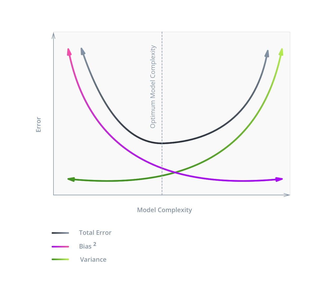
The graph shows that the optimal complexity of the model corresponds to the function C = min (V + B2) , and this value will not correspond to the minimum Bias value.
The complexity of the model consists of two parts. The first part, common to all, is the number of features used (or the dimension of the input data). In our example, there are not many of them, so filtering is unlikely to increase the accuracy of the model, but we will demonstrate the principle itself. In addition, there is always the possibility that some columns may be superfluous, and their removal will not worsen the model. Since, with the same accuracy, a simpler solution should be chosen, even such a change would be useful.
Azure ML has several feature filtering modules for filtering out the least useful ones. We will look at Filter Based Feature Selection .
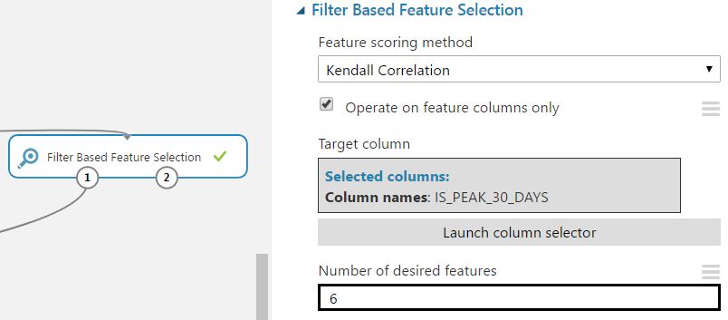
This module includes seven filtering methods: Pearson correlation, mutual information, Kendall correlation, Spearman correlation, chi-squared, Fisher score, count based. Take the Kendall correlation because the data is not normally distributed and does not have a well-defined linear relationship. We set the parameter for the number of desired attributes so that as a result one column is removed.
Let's look at the results of assigning the similarity coefficients of the target and input columns.
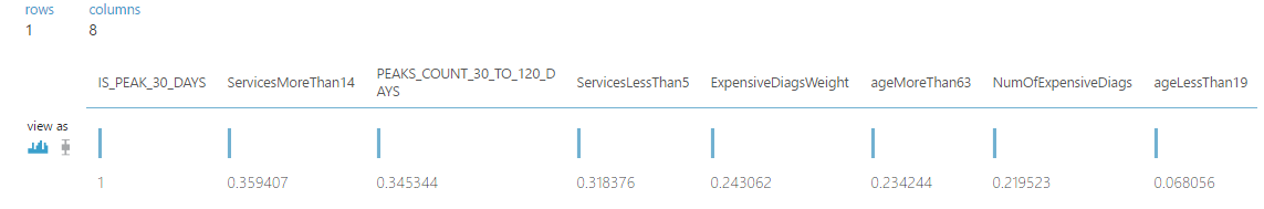
The ageLessThan19 column has a low level of correlation with the target; it can be neglected. Let us verify this by training the Random forest model with the same settings that were used in the example in the previous article .
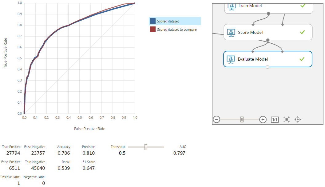
The red curve corresponds to the old model. Removal of the column led to a slight degradation of the model, but within the limits of statistical error. Therefore, the deleted column really had no significant effect on the model and was not needed.
The second part of the complexity of the model depends on the chosen algorithm. In our case, this is a Random forest, for which the complexity is primarily determined by the maximum depth of the trees under construction. Other parameters are also important, but to a lesser extent.
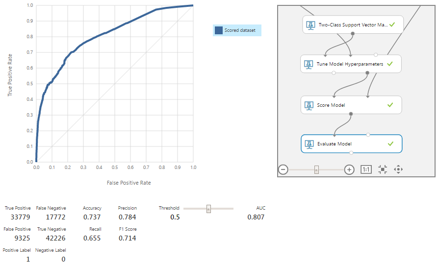
Consider the Azure ML modules that will help with these tasks. For starters, take Tune Model Hyperparameters .
Consider its settings:
The remaining parameters in our case have no meaning or do not require a separate description.
For the module to work correctly in the algorithm initialization, one of the parameters should be changed, the description of which we omitted in the previous article due to its special purpose. It's about create trainer mode . It is necessary to select the parameter range . In this mode, you can select several values for the numerical parameters of the algorithm. Also for each of the numerical parameters you can set the mode range . It is possible to select a range in which potential values will be selected. This is the mode we need - Tune Model Hyperparameters uses these ranges to find the optimal values. In our example, to save time, set the range only for the depth of the decision trees.

Another module that may be useful is Partition and Sample . In assign to folds mode, it breaks data into a specified number of parts. When submitting such input data to the parameter setting module, it begins to work in the cross-validation mode. The remaining settings allow you to specify the number of parts into which the data will be divided, and the features of the partition (for example, an even distribution of values over one of the columns).

With minimal effort, this allowed us to slightly improve our results when evaluating for AUC. With proper settings and a more thorough search for optimal parameters, the improvement in the result will be more substantial.

Now consider another tool for setting up the output model. Since in our case the situation of the binary classification is considered, the belonging to one of the classes is determined through the boundary value. You can check its operation in the Evaluate module tab. At the output of the classifier, we get not a strict class value, but confidence in the presence of a “positive” class, which can take values from 0 to 1. In other words, by default, if the classifier gives a value from 0.5, then in our case the prediction about the presence of a peak will be positive.
Not always 0.5 is the optimal limit. In the case of equivalence of classes, F1 can be a good criterion, although in practice this is rare. Suppose that FN is 2 times more expensive than FP. Consider different boundaries and estimate the total cost for them.
In the graph below, the total cost of FP errors is shown in blue, the color FN in orange, and the sum in green. As you can see, the minimum total cost falls on threshold = 0.31 with a value equal to ≈40.4k. For comparison, at the border equal to 0.5, the price is 15k more.
For clarity, we calculate the minimum cost for a model without a previously removed column.

The illustration shows that the cost is greater. The difference is small, but even such an example is enough to show that more signs do not always give the best model.
Emissions can have a critical impact on model learning outcomes. If the method used is not robust, they can negatively affect the result.
As an example, consider the following case.
Although most of the data is focused on the diagonal, a single point, being far enough away from the others, changes the slope of the function (green). Such points are called high-leverage points. Often they are associated with measurement or recording errors. This is only one of the types of stat emissions and their effect on the model. In our case, the chosen model is robust, so there will be no such influence on it. But to remove the anomalous data in any case is worth it.
To find these points, you can use the Clip Values module. It processes data that goes beyond the designated limits, and can either substitute a different value in it, or mark it as missing. For the purity of the experiment we will conduct this operation only for training records.

Through the module of cleaning the missing values, you can remove rows with missing data, getting an array filtered from anomalies.
Check the accuracy on the new data set.
The model has become a little better in all 4 points. It is worth recalling that the algorithm we are considering is robust. In certain situations, the removal of statistical emissions will give an even greater increase in accuracy.
The committee combines several models into one for better results than each of them can provide. Yes, the algorithm we use is itself a committee, since it consists in building many different decision trees and combining their results into one. However, it is not necessary to stop there.
Consider one of the simplest and, at the same time, popular and effective ways of combining - stacked generalization. Its essence is in using the outputs of different algorithms as attributes for a model of a higher (in terms of hierarchy) level. Like any other committee, it does not guarantee an improvement in the outcome. However, the models obtained through it, as a rule, manifest themselves as more accurate. For our example, let's take a series of algorithms for the binary classification presented in Azure ML Studio: Averaged Perceptron, Bayes Point Machine, Boosted Decision Tree, Random Forest, Decision Jungle and Logistic Regression. At this stage, we will not go into their details - check the work of the committee.
As a result, we obtain one more small improvement of the model for all metrics. Now remember that the classes in our model are not equivalent, and we have accepted that FN is 2 times more expensive than FP. To find the optimal point, check different threshold values.

The minimum amount of the cost of errors is on the border, equal to 0.29, and reaches 40.2. This is only 0.2 less than the figure obtained before the removal of anomalies and calculations through the committee. Of course, much depends on what the real monetary equivalent of this difference will be. But more often, with such a slight improvement, it makes sense to use the principle of Occam's razor and choose a slightly less accurate, but simpler architecture model that we had after adjusting the parameters with the Tune Model Hyperparameters module with a minimum error cost of 40.4.
In the final part of the cycle of articles on machine learning, we examined:
In this series of articles, we presented a simplified version of the cost prediction system, which was implemented as part of a comprehensive solution for an insurance company. On the demonstration model, we described most of the steps necessary to solve problems of this kind: building a prototype, analyzing and processing data, selecting and configuring algorithms, and other tasks.
We also considered one of the most important aspects - the choice of the complexity of the model. The final structure obtained gave the best results in terms of accuracy metrics, f1-score and others. However, when estimating losses from false positive and false negative results, it gave very little profit. In this regard, the less complex model described at the beginning of this article looks more attractive.
These are not all machine learning opportunities in similar tasks, but we have consciously simplified the demonstration model for greater visibility and, in part, due to NDA. The features of the model that are not included in the article are specific to the client’s business and are not well applicable to other projects, since most of the decisions based on machine learning require an individual approach. The full version of the system is used in the real project of our customer, and we continue to improve it.
The WaveAccess team creates technically complex, high-load and fault-tolerant software for companies from different countries. Commentary by Alexander Azarov, Head of Machine Learning at WaveAccess:
The series of articles "Machine learning for an insurance company"
1. Realistic ideas .
2. We investigate the algorithms .
3. Improving the model through algorithm optimization .
Setting the complexity of the model and the boundaries of the definition of classes
Not always the minimum error on the training sample corresponds to the maximum accuracy on the test, since an unnecessarily complex model may lose the ability to generalize.
')
An error in machine learning consists of three parts: Bias , Variance and Noise . With noise ( Noise ), as a rule, nothing can be done: it reflects the influence on the result of factors not considered in the model.
With Bias and Variance, the situation is different. The first displays an error associated with poorly developed dependencies, decreases with increasing complexity and for large values indicates that the model is not sufficiently trained. The second reflects the sensitivity of the model to fluctuations in the values of the input data, increases with increasing complexity and indicates retraining. Hence the concept of bias / variance tradeoff .
The following image illustrates it best:
The graph shows that the optimal complexity of the model corresponds to the function C = min (V + B2) , and this value will not correspond to the minimum Bias value.
The complexity of the model consists of two parts. The first part, common to all, is the number of features used (or the dimension of the input data). In our example, there are not many of them, so filtering is unlikely to increase the accuracy of the model, but we will demonstrate the principle itself. In addition, there is always the possibility that some columns may be superfluous, and their removal will not worsen the model. Since, with the same accuracy, a simpler solution should be chosen, even such a change would be useful.
Azure ML has several feature filtering modules for filtering out the least useful ones. We will look at Filter Based Feature Selection .
This module includes seven filtering methods: Pearson correlation, mutual information, Kendall correlation, Spearman correlation, chi-squared, Fisher score, count based. Take the Kendall correlation because the data is not normally distributed and does not have a well-defined linear relationship. We set the parameter for the number of desired attributes so that as a result one column is removed.
Let's look at the results of assigning the similarity coefficients of the target and input columns.
The ageLessThan19 column has a low level of correlation with the target; it can be neglected. Let us verify this by training the Random forest model with the same settings that were used in the example in the previous article .
The red curve corresponds to the old model. Removal of the column led to a slight degradation of the model, but within the limits of statistical error. Therefore, the deleted column really had no significant effect on the model and was not needed.
The second part of the complexity of the model depends on the chosen algorithm. In our case, this is a Random forest, for which the complexity is primarily determined by the maximum depth of the trees under construction. Other parameters are also important, but to a lesser extent.
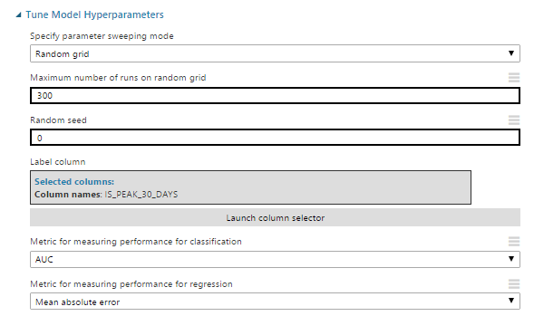
Consider the Azure ML modules that will help with these tasks. For starters, take Tune Model Hyperparameters .
Consider its settings:
- Specify parameter-sweeping mode - set the search mode (in this case, random grid). The search is performed within the values specified at the algorithm initialization stage.
- Maximum number of runs on a random grid - the number of tested options for combinations of parameters for training a model.
- Metric for measuring performance for classification — select from a metric as a target value to optimize classification tasks.
The remaining parameters in our case have no meaning or do not require a separate description.
For the module to work correctly in the algorithm initialization, one of the parameters should be changed, the description of which we omitted in the previous article due to its special purpose. It's about create trainer mode . It is necessary to select the parameter range . In this mode, you can select several values for the numerical parameters of the algorithm. Also for each of the numerical parameters you can set the mode range . It is possible to select a range in which potential values will be selected. This is the mode we need - Tune Model Hyperparameters uses these ranges to find the optimal values. In our example, to save time, set the range only for the depth of the decision trees.
Another module that may be useful is Partition and Sample . In assign to folds mode, it breaks data into a specified number of parts. When submitting such input data to the parameter setting module, it begins to work in the cross-validation mode. The remaining settings allow you to specify the number of parts into which the data will be divided, and the features of the partition (for example, an even distribution of values over one of the columns).
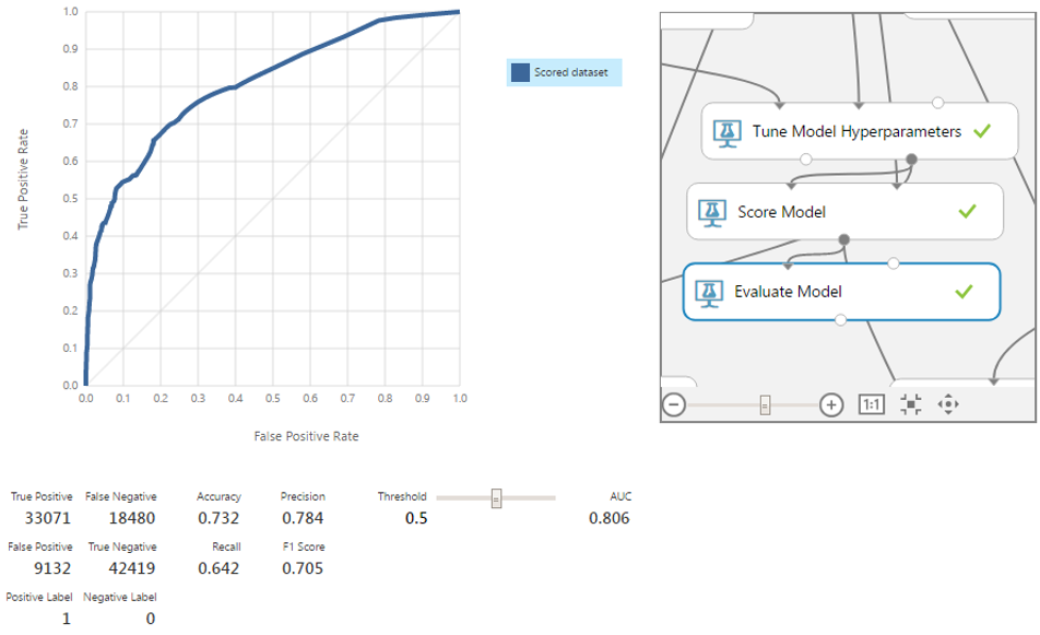
With minimal effort, this allowed us to slightly improve our results when evaluating for AUC. With proper settings and a more thorough search for optimal parameters, the improvement in the result will be more substantial.
Now consider another tool for setting up the output model. Since in our case the situation of the binary classification is considered, the belonging to one of the classes is determined through the boundary value. You can check its operation in the Evaluate module tab. At the output of the classifier, we get not a strict class value, but confidence in the presence of a “positive” class, which can take values from 0 to 1. In other words, by default, if the classifier gives a value from 0.5, then in our case the prediction about the presence of a peak will be positive.
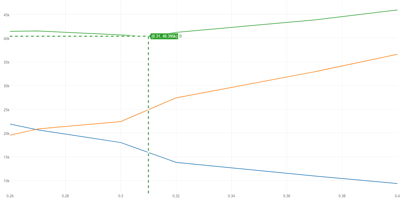
Not always 0.5 is the optimal limit. In the case of equivalence of classes, F1 can be a good criterion, although in practice this is rare. Suppose that FN is 2 times more expensive than FP. Consider different boundaries and estimate the total cost for them.
In the graph below, the total cost of FP errors is shown in blue, the color FN in orange, and the sum in green. As you can see, the minimum total cost falls on threshold = 0.31 with a value equal to ≈40.4k. For comparison, at the border equal to 0.5, the price is 15k more.
For clarity, we calculate the minimum cost for a model without a previously removed column.
The illustration shows that the cost is greater. The difference is small, but even such an example is enough to show that more signs do not always give the best model.
Search for statistical emissions
Emissions can have a critical impact on model learning outcomes. If the method used is not robust, they can negatively affect the result.
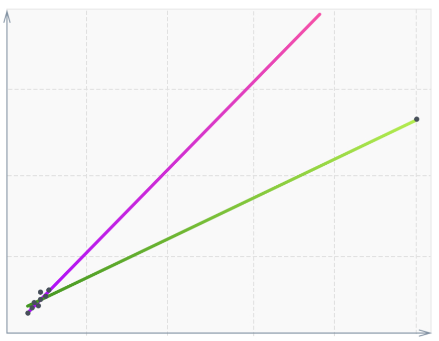
As an example, consider the following case.
Although most of the data is focused on the diagonal, a single point, being far enough away from the others, changes the slope of the function (green). Such points are called high-leverage points. Often they are associated with measurement or recording errors. This is only one of the types of stat emissions and their effect on the model. In our case, the chosen model is robust, so there will be no such influence on it. But to remove the anomalous data in any case is worth it.
To find these points, you can use the Clip Values module. It processes data that goes beyond the designated limits, and can either substitute a different value in it, or mark it as missing. For the purity of the experiment we will conduct this operation only for training records.
Through the module of cleaning the missing values, you can remove rows with missing data, getting an array filtered from anomalies.
Check the accuracy on the new data set.
The model has become a little better in all 4 points. It is worth recalling that the algorithm we are considering is robust. In certain situations, the removal of statistical emissions will give an even greater increase in accuracy.
Use of committee (ensemble) classifiers
The committee combines several models into one for better results than each of them can provide. Yes, the algorithm we use is itself a committee, since it consists in building many different decision trees and combining their results into one. However, it is not necessary to stop there.
Consider one of the simplest and, at the same time, popular and effective ways of combining - stacked generalization. Its essence is in using the outputs of different algorithms as attributes for a model of a higher (in terms of hierarchy) level. Like any other committee, it does not guarantee an improvement in the outcome. However, the models obtained through it, as a rule, manifest themselves as more accurate. For our example, let's take a series of algorithms for the binary classification presented in Azure ML Studio: Averaged Perceptron, Bayes Point Machine, Boosted Decision Tree, Random Forest, Decision Jungle and Logistic Regression. At this stage, we will not go into their details - check the work of the committee.
As a result, we obtain one more small improvement of the model for all metrics. Now remember that the classes in our model are not equivalent, and we have accepted that FN is 2 times more expensive than FP. To find the optimal point, check different threshold values.
The minimum amount of the cost of errors is on the border, equal to 0.29, and reaches 40.2. This is only 0.2 less than the figure obtained before the removal of anomalies and calculations through the committee. Of course, much depends on what the real monetary equivalent of this difference will be. But more often, with such a slight improvement, it makes sense to use the principle of Occam's razor and choose a slightly less accurate, but simpler architecture model that we had after adjusting the parameters with the Tune Model Hyperparameters module with a minimum error cost of 40.4.
Results
In the final part of the cycle of articles on machine learning, we examined:
- Setting the complexity of the model and the choice of the optimal value of the threshold.
- Search and delete statistical emissions from training data.
- Building a committee of several algorithms.
- The choice of the final structure of the model.
In this series of articles, we presented a simplified version of the cost prediction system, which was implemented as part of a comprehensive solution for an insurance company. On the demonstration model, we described most of the steps necessary to solve problems of this kind: building a prototype, analyzing and processing data, selecting and configuring algorithms, and other tasks.
We also considered one of the most important aspects - the choice of the complexity of the model. The final structure obtained gave the best results in terms of accuracy metrics, f1-score and others. However, when estimating losses from false positive and false negative results, it gave very little profit. In this regard, the less complex model described at the beginning of this article looks more attractive.
These are not all machine learning opportunities in similar tasks, but we have consciously simplified the demonstration model for greater visibility and, in part, due to NDA. The features of the model that are not included in the article are specific to the client’s business and are not well applicable to other projects, since most of the decisions based on machine learning require an individual approach. The full version of the system is used in the real project of our customer, and we continue to improve it.
About the authors
The WaveAccess team creates technically complex, high-load and fault-tolerant software for companies from different countries. Commentary by Alexander Azarov, Head of Machine Learning at WaveAccess:
Machine learning allows you to automate areas where expert opinions currently dominate. This makes it possible to reduce the influence of the human factor and increase the scalability of the business.
Source: https://habr.com/ru/post/334556/
All Articles