PyTorch is a modern library of deep learning, developing under the wing of Facebook. It is not similar to other popular libraries, such as Caffe, Theano and TensorFlow. It allows researchers to realize their wildest fantasies, and engineers with ease to implement these fantasies.

This article is a concise introduction to PyTorch and is intended to quickly familiarize yourself with the library and to form an understanding of its main features and its location among other deep learning libraries.

PyTorch is an analogue of the Torch7 framework for the Python language. Its development began in the depths of Facebook back in 2012, just a year after the appearance of Torch7 itself, but PyTorch only became open and accessible to the public in 2017. Since then, the framework is quickly gaining popularity and attracts the attention of an increasing number of researchers. What makes it so popular?

Place among other frameworks

To begin with, let us understand what the deep learning framework is. Deep learning is usually understood to mean the learning of a function that is a composition of a set of non-linear transformations. Such a complex function is also called a flow or computation graph. A deep learning framework should be able to do all three things:

1. Define a calculation graph
2. Differentiate the computation graph;
3. Calculate it.

The faster you know how to calculate your function, and the more flexible your ability to define it, the better. Now, when each framework is able to use all the power of video cards, the first criterion has ceased to play a significant role. What we are really interested in is the available possibilities for defining the flow of calculations. All frameworks here can be divided into three major categories.

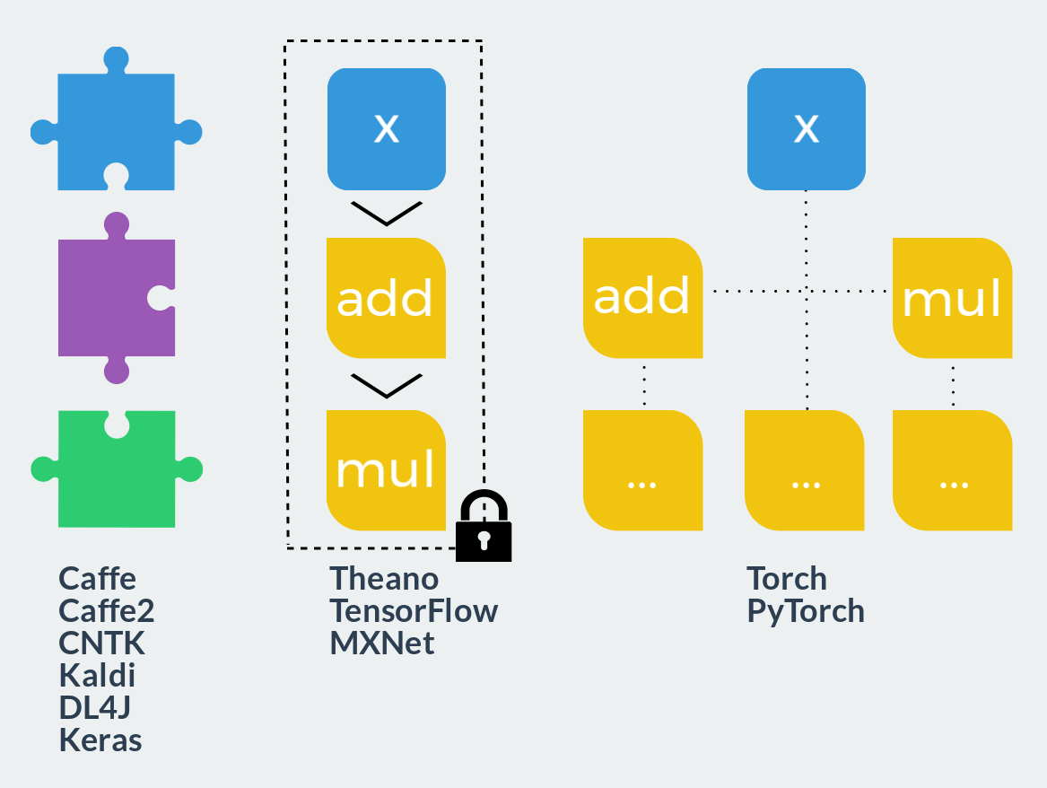
• Fixed modules. This approach can be compared with the Lego constructor: the user combines predefined blocks into a calculation graph and starts it. Forward and reverse passages are already sewn into each such unit. Defining new blocks is much more difficult than using ready-made and requires completely different knowledge and skills. Extensibility is close to zero, but if your ideas are fully implemented in such a framework, the speed of development is maximum. With the speed of work, due to the highly optimized pre-written code, there are also no problems. Typical representatives: Caffe, Caffe2, CNTK, Kaldi, DL4J, Keras (as interface).
• Static calculation graph. These frameworks can already be compared with polymer clay: at the description stage, it is possible to create a graph of calculations of arbitrary size and complexity, but after baking (compilation) it will become solid and solid. Only two actions will remain available: run the graph in forward or reverse directions. All such frameworks use a declarative programming style and resemble functional language or mathematical notation. On the one hand, this approach combines flexibility at the design stage and speed at the time of execution. On the other hand, as in functional languages, debugging becomes a real headache, and models that go beyond the paradigm require either titanic efforts or hefty crutches to implement. Representatives: Theano, TensorFlow, MXNet.
• Dynamic computation graph. Imagine now that you can rebuild a static graph before each run. This is approximately what happens in this class of frameworks. Only the graph as a separate entity is not here. It, as well as in imperative programming languages, is too complex for explicit construction and exists only at the time of execution. More precisely, the graph is built dynamically each time with a direct pass in order to then be able to make the pass reverse. Such an approach gives maximum flexibility and extensibility, allows using all the capabilities of the programming language used in calculations and does not limit the user to anything at all. This class of frameworks includes Torch and PyTorch.

I am sure many of us began to deal with deep learning, using only NumPy. A direct passage is trivial to write on it, and the formula for updating the scales can be calculated on a piece of paper or even get ready weights from the astral. This first code could look like this:

import numpy as np def MyNetworkForward(weights, bias, x): h1 = weights @ x + bias a1 = np.tanh(h1) return a1 y = MyNetworkForward(weights, bias, x) loss = np.mean((y - y_hat) ** 2) 

Over time, network architectures become more complex and deeper, and the possibilities of NumPy, pencil and paper, are no longer enough. If your connection with the astral has not yet been closed by this time and you have a place to take weight, you are lucky. Otherwise, involuntarily you begin to think about two things:

1. That would be able to run my calculations on the video card;
2. That would be all gradients considered for me.

You do not want to change the usual approach, just want to write:

 import numpy as np def MyNetworkForward(weights, bias, x): h1 = weights @ x + bias a1 = np.tanh(h1) return a1 weights.cuda() bias.cuda() x.cuda() y = MyNetworkForward(weights, bias, x) loss = np.mean((y - y_hat) ** 2) loss.magically_calculate_backward_pass() 

Well, guess what? PyTorch does exactly that! Here is a completely correct code:

 import torch def MyNetworkForward(weights, bias, x): h1 = weights @ x + bias a1 = torch.tanh(h1) return a1 weights = weights.cuda() bias = bias.cuda() x = x.cuda() y = MyNetworkForward(weights, bias, x) loss = torch.mean((y - y_hat) ** 2) loss.backward() 

It remains only to apply the already calculated parameter updates.

In Theano and TensorFlow, we describe a graph on a declarative DSL, which is then compiled into some internal bytecode and executed in a monolithic kernel written in C ++, or compiled into C code and executed as a separate binary object. If at the moment of compilation we know the entire graph as a whole, we can easily differentiate it, for example, symbolically. However, is the compilation stage necessary?

It turns out no. Nothing prevents us from building a graph dynamically simultaneously with its calculation! And thanks to the automatic differentiation technique (automatic differentiation, AD), we can take and differentiate the graph at any time in any state. There is absolutely no real need to compile a graph. As for speed, calling lightweight native procedures from the Python interpreter is no slower than executing compiled code.

Not limited to DSL and compilation, we can use all the features of Python and make the code truly dynamic. For example, use different activation functions on even and odd days:

 from datetime import date import torch.nn.functional as F ... if date.today().day % 2 == 0: x = F.relu(x) else: x = F.linear(x) ... 

Or we can create a layer that each time adds the value just entered by the user to the tensor:

 ... x += int(input()) ... 

I will show a more useful example at the end of the article. In summary, all of the above can be expressed by the following formula:
PyTorch = NumPy + CUDA + AD .

Tensor calculations

Let's start with the numpy part. Tensor calculations are the basis of PyTorch, a framework around which all other functionality is built up. Unfortunately, it is impossible to say that the power and expressiveness of the library in this aspect coincides with that of NumPy. In all that relates to working with tensors, PyTorch is guided by the principle of maximum simplicity and transparency, providing a thin wrapper over BLAS calls.

Tensors

The type of data stored by the tensor is reflected in the name of its constructor. A constructor without parameters will return a special value — a tensor without dimension, which cannot be used in any operations.

 >>> torch.FloatTensor() [torch.FloatTensor with no dimension] 

All possible types:

 torch.HalfTensor # 16 ,    torch.FloatTensor # 32 ,    torch.DoubleTensor # 64 ,    torch.ShortTensor # 16 , ,  torch.IntTensor # 32 , ,  torch.LongTensor # 64 , ,  torch.CharTensor # 8 , ,  torch.ByteTensor # 8 , ,  

No automatic type detection or default type exists. torch.Tensor is a short name for torch.FloatTensor .

The automatic type casting in NumPy is also not performed:

 >>> a = torch.FloatTensor([1.0]) >>> b = torch.DoubleTensor([2.0]) >>> a * b 

 TypeError: mul received an invalid combination of arguments - got (torch.DoubleTensor), but expected one of: * (float value) didn't match because some of the arguments have invalid types: (torch.DoubleTensor) * (torch.FloatTensor other) didn't match because some of the arguments have invalid types: (torch.DoubleTensor) 

In this regard, PyTorch stricter and safer: you will not stumble upon a twofold increase in memory consumption, confusing the type of constant. Explicit type casting is available using methods with appropriate names.

 >>> a = torch.IntTensor([1]) >>> a.byte() 1 [torch.ByteTensor of size 1] >>> a.float() 1 [torch.FloatTensor of size 1] 

x.type_as(y) returns the tensor of values ​​from x the same type as y .

Any coercion of a tensor to its own type does not copy it.

If we transfer the list to the constructor of the tensor as a parameter, we construct the tensor of the corresponding dimension and the corresponding data.

 >>> a = torch.IntTensor([[1, 2], [3, 4]]) >>> a 1 2 3 4 [torch.IntTensor of size 2x2] 

Malformed lists are not allowed in the same way as in NumPy.

 >>> torch.IntTensor([[1, 2], [3]]) 

 RuntimeError: inconsistent sequence length at index (1, 1) - expected 2 but got 1 

It is allowed to construct a tensor from the value of any type of sequence , which is very intuitive and corresponds to the behavior of NumPy.

Another possible set of arguments of the tensor constructor is its size. The number of arguments determines the dimension.

The tensor constructed by this method contains garbage - random values.

 >>> torch.FloatTensor(1) 1.00000e-17 * -7.5072 [torch.FloatTensor of size 1] 

 >>> torch.FloatTensor(3, 3) -7.5072e-17 4.5909e-41 -7.5072e-17 4.5909e-41 -5.1601e+16 3.0712e-41 0.0000e+00 4.5909e-41 6.7262e-44 [torch.FloatTensor of size 3x3] 

Indexing

Standard Python indexing is supported: indexing and slicing.

 >>> a = torch.IntTensor([[1, 2, 3], [4, 5, 6]]) >>> a 1 2 3 4 5 6 [torch.IntTensor of size 2x3] 

 >>> a[0] 1 2 3 [torch.IntTensor of size 3] 

 >>> a[0][1] 2 >>> a[0, 1] 2 

 >>> a[:, 0] 1 4 [torch.IntTensor of size 2] >>> a[0, 1:3] 2 3 [torch.IntTensor of size 2] 

Also, other tensors can act as indices. However, there are only two possibilities here:

• One-dimensional torch.LongTensor , indexing by zero dimension (by elements in the case of vectors and by rows in the case of matrices);
• A commensurate torch.ByteTensor , containing only 0 or 1 values ​​that serves as a mask.

 >>> a = torch.ByteTensor(3,4).random_() >>> a 26 119 225 238 83 123 182 83 136 5 96 68 [torch.ByteTensor of size 3x4] >>> a[torch.LongTensor([0, 2])] 81 218 40 131 144 46 196 6 [torch.ByteTensor of size 2x4] 

 >>> a > 128 0 1 0 1 0 0 1 0 1 0 1 0 [torch.ByteTensor of size 3x4] >>> a[a > 128] 218 131 253 144 196 [torch.ByteTensor of size 5] 

The x.dim() , x.size() and x.type() functions will help you to find all the available information about the tensor, and x.data_ptr() will indicate the place in memory where the data is located.

 >>> a = torch.Tensor(3, 3) >>> a.dim() 2 >>> a.size() torch.Size([3, 3]) >>> a.type() 'torch.FloatTensor' >>> a.data_ptr() 94124953185440 

Operations on tensors

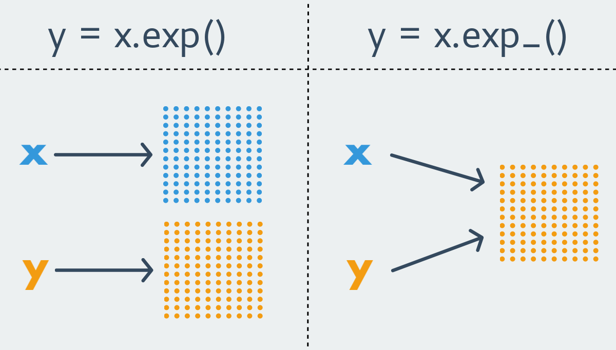
The PyTorch naming convention states that any function of the form xxx returns a new tensor, i.e. is immutable function. In contrast, a function of the form xxx_ changes the initial tensor, i.e. is a mutable function. The latter are also called inplace functions.

For almost any immutable function in PyTorch, there is its less pure counterpart. However, it also happens that the function exists only in one variant. For obvious reasons, functions that change the size of the tensor are always immutable.

I will not list all the available operations on tensors, I’ll dwell only on the most important ones and divide them into categories.

Initialization functions

As a rule, they are used for initialization when creating new tensors of a given size.

 x = torch.FloatTensor(3, 4) #  x.zero_() #  

Since the mutable functions return an object reference, it is more convenient to write the declaration and initialization in one line.

 x = torch.FloatTensor(3, 4).zero_() 

• x.zero_()
  Initializes the tensor with zeros. Does not have an immutable option.
• x.fill_(n)
  Fills the tensor with the constant n. Similarly, it does not have an immutable option.
• x.random_(from, to)
  Fills the tensor with samples from discrete (even for real-valued tensors) uniform distribution.
  

  If from and to not specified, they are equal to the lower and upper bounds of the used data type, respectively.
  

• x.uniform_(from=0, to=1)
  Also a uniform distribution, but already continuous and with more familiar boundaries by default. Only available for real-valued tensors.
• x.normal_(mean=0, std=1)
  Normal distribution. Only available for real-valued tensors.
• x.bernoulli_(p=0.5)
  Bernoulli distribution. As p , a scalar or a tensor of the same dimension with the values 0 <= p <= 1 can be used. It is important to distinguish this version from the immutable version, since it has a different semantics. Calling y = x.bernoulli() equivalent to y.bernoulli_(x) , i.e. x itself is used here as a tensor of distribution parameters.
• torch.eye(n, m)
  Creates the nxm identity matrix. Here, for reasons that are not clear to me, the option inplace does not already exist.

Exponential and geometric distributions, the Cauchy distribution, the logarithm of the normal distribution, and several more complex tensor initialization options are also available. Feel free to look into the documentation!

Mathematical operations

The most frequently used group. If the operation here does not change the size and type of the tensor, then it has an inplace option.

• z = x.add(y)
z = torch.add(x, y)
x.add_(y)
  Addition.
• z = x.sub(y)
z = torch.sub(x, y)
x.sub_(y)
  Subtraction
• z = x.mul(y)
z = torch.mul(x, y)
x.mul_(y)
  Multiplication.
• z = x.div(y)
z = torch.div(x, y)
x.div_(y)
  Division. For integer types, division is integer.
• z = x.exp()
z = torch.exp(x)
x.exp_()
  Exhibitor.
• z = x.log()
z = torch.log(x)
x.log_()
  Natural logarithm.
• z = x.log1p()
z = torch.log1p(x)
x.log1p_()
  The natural logarithm of x + 1 . The function is optimized for accuracy of calculations for small x .
• z = x.abs()
z = torch.abs(x)
x.abs_()
  Module.

Naturally, there are all the basic trigonometric operations in the form in which you expect to see them. We now turn to less trivial functions.

• z = xt()
z = torch.t(x)
x.t_()
  Transposing. Despite the fact that the size of the tensor varies, there is an inplace version of the function, since the size of the data in memory remains the same.
• z = x.mm(y)
z = torch.mm(x, y)
  Matrix multiplication.
• z = x.mv(v)
z = torch.mv(x, v)
  Matrix multiplication by vector.
• z = x.dot(y)
z = torch.dot(x, y)
  Scalar multiplication of tensors.
• bz = bx.bmm(by)
bz = torch.bmm(bx, by)
  Multiplies matrices with whole batch.
  

   >>> bx = torch.randn(10, 3, 4) >>> by = torch.randn(10, 4, 5) >>> bz = bx.bmm(bz) >>> bz.size() torch.Size([10, 3, 5]) 

There are also complete analogs of BLAS functions with complex signatures, such as addbmm , addmm , addmv , addr , baddbmm , btrifact , btrisolve , eig , gels and many others.

The operations of reduction are similar to each other by signature. Almost all of them, with their last optional argument, take dim , the dimension in which the reduction is performed. If the argument is not specified, the operation affects the entire tensor as a whole.

• s = x.mean(dim)
s = torch.mean(x, dim)
  Selective average. Defined only for real-valued tensors.
• s = x.std(dim)
s = torch.std(x, dim)
  Selective standard deviation. Defined only for real-valued tensors.
• s = x.var(dim)
s = torch.var(x, dim)
  Selective dispersion. Defined only for real-valued tensors.
• s = x.median(dim)
s = torch.median(x, dim)
  Median.
• s = x.sum(dim)
s = torch.sum(x, dim)
  Amount.
• s = x.prod(dim)
s = torch.prod(x, dim)
  Composition.
• s = x.max(dim)
s = torch.max(x, dim)
  Maximum.
• s = x.min(dim)
s = torch.min(x, dim)
  Minimum.

Various comparison operations ( eq , ne , gt , lt , ge , le ) are also defined and return as a result of their work a mask of the type ByteTensor .

The operators + , += , - , -= , * , *= , / , /= , @ work exactly as you would expect, calling the corresponding functions described above. However, due to the complexity and incomplete evidence of the API, I do not recommend using operators, but use an explicit call of the necessary functions instead. At least you should not mix two styles, this will avoid errors like x += x.mul_(2) .

PyTorch still has many interesting functions in stock, such as sorting or elementwise function, but they are rarely used in deep learning. If you want to use PyTorch as a library of tensor calculations, do not forget to look into the documentation before.

Broadcasting

Broadcasting is a complex topic. In my opinion, it would have been better. But it is, although it appeared only in one of the latest releases. Many operations in PyTorch now support broadcasting in the usual NumPy style.

Generally speaking, two non-empty tensors are called broadcastable , if, starting from the last measurement, the dimensions of both tensors in this dimension are either equal, or the size of one of them is equal to one, or measurements in the tensor no longer exist. Easier to understand with examples.

 >>> x = torch.FloatTensor(5, 7, 3) >>> y = torch.FloatTensor(5, 7, 3) # broadcastable,  :  ,    ,  

 >>> x = torch.FloatTensor(5, 3, 4, 1) >>> y = torch.FloatTensor( 3, 1, 1) # broadcastable,     ,         ,     ,        

 >>> x = torch.FloatTensor(5, 2, 4, 1) >>> y = torch.FloatTensor( 3, 1, 1) #  broadcastable,       (2 != 3)            

 >>> x = torch.FloatTensor() >>> y = torch.FloatTensor(2, 2) #  broadcastable,  x     ()  

The tensor of dimension torch.Size([1]) , being a scalar, is obviously broadcastable with any other tensor.

The size of the tensor resulting from broadcasting is calculated as follows:

1. If the number of measurements of the tensors is not equal, then where necessary, units are added.
2. Then the size of the resulting tensor is calculated as the elementwise maximum of the initial tensors.

 >>> x = torch.FloatTensor(5, 1, 4, 1) >>> y = torch.FloatTensor( 3, 1, 1) >>> (x+y).size() torch.Size([5, 3, 4, 1]) 

In the example, the dimension of the second tensor was supplemented with a unit at the beginning, and then the elementwise maximum determined the dimension of the resulting tensor.

The catch lies in inplace operations. Broadcasting is allowed for them only when the size of the original tensor does not change.

 >>> x = torch.FloatTensor(5, 3, 4, 1) >>> y = torch.FloatTensor( 3, 1, 1) >>> (x.add_(y)).size() torch.Size([5, 3, 4, 1]) 

 >>> x=torch.FloatTensor(1, 3, 1) >>> y=torch.FloatTensor(3, 1, 7) >>> (x.add_(y)).size() 

 RuntimeError: The expanded size of the tensor (1) must match the existing size (7) at non-singleton dimension 2. 

In the second case, the tensors are obviously broadcastable, but the inplace operation is not allowed, since x would change its size during it.

From NumPy and back

The functions torch.from_numpy(n) and x.numpy() can be used to convert tensors from one library to tensors of another.

Tensors at the same time use the same internal storage, copying data does not occur.

 >>> import torch >>> import numpy as np >>> a = np.random.rand(3, 3) >>> a array([[ 0.3191423 , 0.75283128, 0.31874139], [ 0.0077988 , 0.66912423, 0.3410516 ], [ 0.43789109, 0.39015864, 0.45677317]]) >>> b = torch.from_numpy(a) >>> b 0.3191 0.7528 0.3187 0.0078 0.6691 0.3411 0.4379 0.3902 0.4568 [torch.DoubleTensor of size 3x3] >>> b.sub_(b) 0 0 0 0 0 0 0 0 0 [torch.DoubleTensor of size 3x3] >>> a array([[ 0., 0., 0.], [ 0., 0., 0.], [ 0., 0., 0.]]) 

That's all the main points of the PyTorch tensor library are suggested to be considered. I hope now it’s clear to the reader that implementing a straight pass for an arbitrary function on PyTorch is just as easy as using NumPy. It is only necessary to get used to the inplace operations and remember the names of the main functions. For example, the linear layer with the softmax activation function:

 def LinearSoftmax(x, w, b): s = x.mm(w).add_(b) s.exp_() s.div_(s.sum(1)) return s 

CUDA

Everything is simple here: tensors can live either "on the processor" or "on the video card." True, they are very picky and live only on video cards from Nvidia, and not on the oldest. By default, a tensor is created on the CPU.

 x = torch.FloatTensor(1024, 1024).uniform_() 

The memory of the video card is empty.

 0MiB / 4036MiB 

In one call, we can move the tensor to the GPU.

 x = x.cuda() 

In this case, nvidia-smi will show that the python process took up some amount of video memory.

 205MiB / 4036MiB 

The x.is_cuda property helps to understand where the tensor x is now.

 >>> x.is_cuda True 

In fact, x.cuda() returns a copy of the tensor, rather than moving it.

When all references to a tensor in video memory disappear, PyTorch will not delete it instantly. Instead, the next time he allocates it, he will either reuse this section of the video memory or clear it.

If you have several video cards, the x.cuda(device=None) function x.cuda(device=None) will gladly accept as an optional argument the number of the video card where the tensor should be placed, and the x.get_device() function will show on which device the tensor x is. The x.cpu() function copies the tensor from the video card "to the processor".

Naturally, we cannot perform any operations with tensors located on different devices.

Here, for example, how to multiply two tensors on a video card and return the result back to RAM:

 >>> import torch >>> a = torch.FloatTensor(10000, 10000).uniform_() >>> b = torch.FloatTensor(10000, 10000).uniform_() >>> c = a.cuda().mul_(b.cuda()).cpu() 

And all this is available directly from the interpreter! Present a similar code on TensorFlow, where you have to create a graph, session, compile a graph, initialize the variables and run the graph in a session. With PyTorch, I can even sort the tensor on a video card with a single line of code!

Tensors can not only be copied to a video card, but also created directly on it. This is done using the torch.cuda module.

There torch.cuda no abbreviation for Tensor = FloatTensor .

The context manager torch.cuda.device(device) allows you to create all the tensors defined inside it on a specified video card. The results of operations on tensors from other devices will remain where they should be. The value transferred to x.cuda(device=None) is more priority than that dictated by the context manager.

 x = torch.cuda.FloatTensor(1) # x.get_device() == 0 y = torch.FloatTensor(1).cuda() # y.get_device() == 0 with torch.cuda.device(1): a = torch.cuda.FloatTensor(1) # a.get_device() == 1 b = torch.FloatTensor(1).cuda() # a.get_device() == b.get_device() == 1 c = a + b # c.get_device() == 1 z = x + y # z.get_device() == 0 d = torch.FloatTensor(1).cuda(2) # d.get_device() == 2 

The x.pin_memory() function, available only for tensors on the CPU, copies the tensor to the page-locked memory area. Its peculiarity is that the data from it can be very quickly copied to the GPU without the participation of the processor. The x.is_pinned() method will display the current status of the tensor. After the tensor is in page-locked memory, we can pass the named parameter async=True to x.cuda(device=None, async=False) to ask it to load the tensor onto the video card asynchronously. Thus, your code can not wait for the completion of copying and do something useful during this time.

The async parameter has no effect if x.is_pinned() == False . Errors this, too, will not cause.

As you can see, the adaptation of your arbitrary code for computing on a video card only requires copying all the tensors into the video memory. Most operations do not matter where your tensors are located, if they are on the same device.

Automatic differentiation

The mechanism of automatic differentiation, contained in the module torch.autograd , is, though not the main one, but, undoubtedly, the most important component of the library, without which it would lose all meaning.

Calculating the gradient of a function at a given point is the central operation of optimization methods, which, in turn, keeps all deep learning. Learning here is synonymous with optimization. There are three main ways to calculate the gradient of a function at a point:

1. Numerically by the finite difference method;
2. Symbolically;
3. Use the technique of automatic differentiation.

The first method is used only to verify the results due to its low accuracy. Symbolic calculation of the derivative is equivalent to what you do manually, using paper and pencil, and is to apply the list of rules to the tree of characters. About automatic differentiation, I will describe in the following paragraphs. Libraries like Caffe and CNTK use a predefined derived function in symbolic form. Theano and TensorFlow use a combination of methods 2 and 3.

Automatic differentiation (AD) is a fairly simple and very obvious technique for calculating the gradient of a function. If you, without using the Internet, try to solve the problem of differentiating a function at a given point, you will definitely come to AD.

This is how AD works. Any of the functions of interest to us can be expressed as a composition of some elementary functions whose derivatives are known to us. Then, using the rule of differentiation of a complex function, we can rise higher and higher, until we arrive at the desired derivative. For example, consider the function of two variables

$$

$$f (x_1, x_2) = x_1 x_2 + x_1 ^ 2.$$

Redefine

$$

$$w_1 = x_1,$$

$$

$$w_2 = x_2,$$

$$

$$w_3 = w_1 w_2,$$

$$

$$w_4 = w_1 ^ 2,$$

$$

$$w_5 = w_3 + w_4.$$

— .

,

$$

$$\dfrac{\partial{f(x_1^*, x_2^*)}}{\partial{x_1}}.$$

$$

$$\dfrac{\partial{f}}{\partial{x_1}} = \dfrac{\partial{f}}{\partial{w_5}} \dfrac{\partial{w_5}}{\partial{x_1}} = \dfrac{\partial{f}}{\partial{w_5}} \Big[ \dfrac{\partial{w_5}}{\partial{w_4}} \dfrac{\partial{w_4}}{\partial{x_1}} + \dfrac{\partial{w_5}}{\partial{w_3}} \dfrac{\partial{w_3}}{\partial{x_1}} \Big] = \cdots$$

— — . . , — .

$$

$$\dfrac{\partial{w_1(x_1^*, x_2^*)}}{\partial{x_1}} = 1$$

$$

$$\dfrac{\partial{w_2(x_1^*, x_2^*)}}{\partial{x_1}} = 0$$

$$

$$\dfrac{\partial{w_3(x_1^*, x_2^*)}}{\partial{x_1}} = \dfrac{\partial{w_1(x_1^*, x_2^*)}}{\partial{x_1}} w_2 + \dfrac{\partial{w_2(x_1^*, x_2^*)}}{\partial{x_1}} w_1 = x_2^*$$

$$

$$\dfrac{\partial{w_4(x_1^*, x_2^*)}}{\partial{x_1}} = 2 w_1\dfrac{\partial{w_1(x_1^*, x_2^*)}}{\partial{x_1}} = 2 x_1^*$$

$$

$$\dfrac{\partial{w_5(x_1^*, x_2^*)}}{\partial{x_1}} = \dfrac{\partial{w_3(x_1^*, x_2^*)}}{\partial{x_1}} + \dfrac{\partial{w_4(x_1^*, x_2^*)}}{\partial{x_1}} = x_2^* + 2 x_1^*$$

$$

$$\dfrac{\partial{f(x_1^*, x_2^*)}}{\partial{x_1}} = \dfrac{\partial{f(x_1^*, x_2^*)}}{\partial{w_5}} \dfrac{\partial{w_5(x_1^*, x_2^*)}}{\partial{x_1}} = x_2^* + 2 x_1^*$$

. , . , — , . , — .

AD, 20 Python! . .

 class Varaible: def __init__(self, value, derivative): self.value = value self.derivative = derivative 

, , .

  def __add__(self, other): return Varaible( self.value + other.value, self.derivative + other.derivative ) 

  def __mul__(self, other): return Varaible( self.value * other.value, self.derivative * other.value + self.value * other.derivative ) def __pow__(self, other): return Varaible( self.value ** other, other * self.value ** (other - 1) ) 

x1 .

 def f(x1, x2): vx1 = Varaible(x1, 1) vx2 = Varaible(x2, 0) vf = vx1 * vx2 + vx1 ** 2 return vf.value, vf.derivative print(f(2, 3)) # (10, 7) 

Variable torch.autograd . , , , PyTorch . , , . Let's take an example.

 >>> from torch.autograd import Variable >>> x = torch.FloatTensor(3, 1).uniform_() >>> w = torch.FloatTensor(3, 3).uniform_() >>> b = torch.FloatTensor(3, 1).uniform_() >>> x = Variable(x, requires_grad=True) >>> w = Variable(w) >>> b = Variable(b) >>> y = w.mv(x).add_(b) >>> y Variable containing: 0.7737 0.6839 1.1542 [torch.FloatTensor of size 3] >>> loss = y.sum() >>> loss Variable containing: 2.6118 [torch.FloatTensor of size 1] >>> loss.backward() >>> x.grad Variable containing: 0.2743 1.0872 1.6053 [torch.FloatTensor of size 3] 

: Variable , . x.backward() , requires_grad=True . x.grad . x.data .

, Variable .

x.requires_grad , . : , .

, inplace . , , Variable , . : , immutable . mutable . : PyTorch -, .

Example

FaceResNet-1337 . PyTorch, , , . , .

, Deep Function Machines: Generalized Neural Networks for Topological Layer Expression . . , . , , , . :

$$

$$V_n(v) = \int_n^{n+1} (u - n) w_l(u, v) d \mu(u)$$

$$

$$Q_n(v) = \int_n^{n+1} w_l(u, v) d \mu(u)$$

$$

$$W_{n,j} = Q_n(j) - V_n(j) + V_{n-1}(j)$$

$$

$$W_{N, j} = V_{N-1}(j)$$

$$

$$W_{1,j} = Q_1(j) - V_1(j)$$

. w — , W — , . W , - , , w . ? PyTorch — . .

 import numpy as np import torch from torch.autograd import Variable def kernel(u, v, s, w, p): uv = Variable(torch.FloatTensor([u, v])) return s[0] + w.mv(uv).sub_(p).cos().dot(s[1:]) 

.

 def integrate(fun, a, b, N=100): res = 0 h = (b - a) / N for i in np.linspace(a, b, N): res += fun(a + i) * h return res 

.

 def V(v, n, s, w, p): fun = lambda u: kernel(u, v, s, w, p).mul_(u - n) return integrate(fun, n, n+1) def Q(v, n, s, w, p): fun = lambda u: kernel(u, v, s, w, p) return integrate(fun, n, n+1) def W(N, s, w, p): Qp = lambda v, n: Q(v, n, s, w, p) Vp = lambda v, n: V(v, n, s, w, p) W = [None] * N W[0] = torch.cat([Qp(v, 1) - Vp(v, 1) for v in range(1, N + 1)]) for j in range(2, N): W[j-1] = torch.cat([Qp(v, j) - Vp(v, j) + Vp(v, j - 1) for v in range(1, N + 1)]) W[N-1] = torch.cat([ Vp(v, N-1) for v in range(1, N + 1)]) W = torch.cat(W) return W.view(N, N).t() 

.

 s = Variable(torch.FloatTensor([1e-5, 1, 1]), requires_grad=True) w = Variable(torch.FloatTensor(2, 2).uniform_(-1e-5, 1e-5), requires_grad=True) p = Variable(torch.FloatTensor(2).uniform_(-1e-5, 1e-5), requires_grad=True) 

.

 data_x_t = torch.FloatTensor(100, 3).uniform_() data_y_t = data_x_t.mm(torch.FloatTensor([[1, 2, 3]]).t_()).view(-1) 

.

 alpha = -1e-3 for i in range(1000): data_x, data_y = Variable(data_x_t), Variable(data_y_t) Wc = W(3, s, w, p) y = data_x.mm(Wc).sum(1) loss = data_y.sub(y).pow(2).mean() print(loss.data[0]) loss.backward() s.data.add_(s.grad.data.mul(alpha)) s.grad.data.zero_() w.data.add_(w.grad.data.mul(alpha)) w.grad.data.zero_() p.data.add_(p.grad.data.mul(alpha)) p.grad.data.zero_() 

. .

. 3d matplotlib , . , , , 15 . . TensorFlow… , TensorFlow. PyTorch . , PyTorch . , PyTorch , .

.

 data_x, data_y = Variable(data_x_t), Variable(data_y_t) 

, . - , , : .

 loss.backward() 

, , .

 s.data.add_(s.grad.data.mul(alpha)) 

(), . .

 s.grad.data.zero_() 

backward() , .

, : PyTorch , , , Keras.

Conclusion

PyTorch: , cuda . PyTorch .

, PyTorch . , . : PyTorch , . , Caffe, DSL TensorFlow. PyTorch , , .

, , torch.nn torch.optim . torch.utils.data . torchvision . .

PyTorch . . - . , . .

! , , , . .