The ghost of a locomotive or the stock market through the prism of correlations
This article will demonstrate the technique of processing information on stock quotes using the pandas (python) package, as well as studying some of the “myths and legends” of stock trading through the use of mathematical statistics methods. Along the way, let's briefly review the features of using the plotly library.
One of the legends of traders is the concept of "locomotive". It can be described as follows: there are “lead” papers and there are “follower” papers. If we believe in the existence of such a pattern, then we can “predict” the future movements of a financial instrument along the movement of “locomotives” (“leading” securities). Is it so? Is there a reason for this?

We formulate the problem. There are financial instruments: A, B, C, D; there is a time characteristic - t. Are there any links between the movements of these tools:
A t and B t-1 ; A t and C t-1 ; A t and D t-1
B t and C t-1 ; B t and D t-1 ; B t and A t-1
C t and D t-1 ; C t and A t-1 ; C t and B t-1
D t and A t-1 ; D t and B t-1 ; D t and B t-1
')
How to get data for the study of this issue? How strong, stable are the links mentioned? How can they be measured? What tools?
 We first note that today there are a significant number of predictive models. Some sources say that their number has exceeded one hundred . By the way - the main joke of reality is that ... the more complex the model, the harder the interpretation, the understanding of each individual component of this model itself. I emphasize that the purpose of this article is to answer the above questions , and not to use one of the existing forecasting models.
The pandas package is a powerful data analysis tool that has a rich arsenal of tools. We use its capabilities to study the questions raised by us.
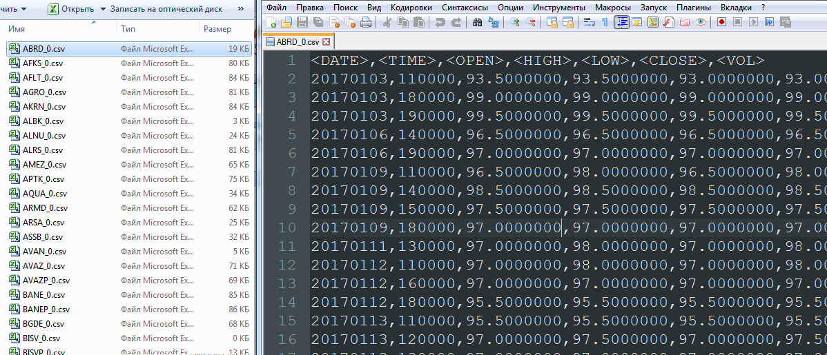
Previously, we get quotes from the server of the company "FINAM". We will take the "watch" for the period from 01/01/2017 to 13/07/2017 . By slightly modifying the function mentioned here , we get:
As a result, we have a list of files of type A_0.csv:
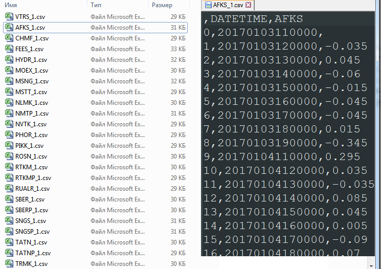
Next, we determine the movements of financial instruments A t -A t-1 , remove the columns OPEN, HIGH, LOW, VOL, form a single column DATETIME. We will eliminate those financial instruments that have too little data for analysis (they are traded recently, unstable or have low liquidity).
As a result, we get a list of files of type A_1.csv. Total 91 files:
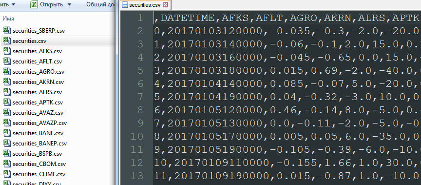
We merge all movements of all financial instruments into one file securities.csv by deleting the first empty line.
At this stage, there is a rather interesting operation of merging records by the DATETIME column (pd.merge). This merger procedure discards those dates on which at least one of the 91 securities did not trade. That is, the union is based on the complete elimination of empty data. As a result:
In the file securities.csv , operating with data in a cycle, we shift all lines except the current one. Thus, on the contrary A t are the values B t-1 , C t-1 , D t-1 .
The data will look like this:

And yes, you need to delete the first row with empty data. Now you can build correlations between columns. They will then reveal the existence or absence of papers, “locomotives” ... or they will make it possible to make sure that “locomotives” are nothing more than a myth.
The fact of the absence of a normal (Gaussian) distribution in the movement of financial instruments is mentioned relatively recently. Nevertheless, the majority of financial models are based on his assumption. Is the Gaussian distribution present in our data? The question is not idle, since the existence of normality will allow the use of the Pearson correlation, and the absence will oblige the use of a nonparametric form of correlation. With this question we turn to plotly's wonderful service.
 What is interesting this service? Firstly, the ability to graphically interpret the data. Secondly, a set of statistical test methods; in particular, the possibility of conducting tests for the conformity of the sample to the normal (Gaussian) distribution. We will use the following tests: the Shapiro-Wilk criterion (Shapiro-Wilk), the Kolmogorov-Smirnov criterion (Kolmogorov-Smirnov), see the rules of work here .
The service related to plotly is worthy of the highest praise. Tutorial on setting up plotly on Linux can be viewed on plot.ly, and under Windows, for example, here . But there are plotly and weirdness. And the question here is nothing more than a description of the logic of the test. In the examples for the application table is given:

The developer gives the following comment:
Since our p-value is less than our test status, the numerical hypothesis at the 0.05 significance level.
Transfer:
Since our p-value is much smaller than our test statistics, we have good evidence that we do not reject the null hypothesis at the 0.05 significance level.
Thus, according to this recommendation, we are not entitled to abandon the hypothesis of normal distribution for the sample under consideration! But ... this advice is not correct .
So, remember - what is p-value? This value is necessary for testing statistical hypotheses. It can be understood as the probability of error if we reject the null hypothesis. Under the null hypothesis in the Shapiro-Wilk criterion H 0 , I recall, it means that "the random variable X is distributed normally." If we reject H 0 for an extremely small p-value (close to zero), then we will not be mistaken. We are not mistaken in eliminating the assumption of normal distribution. In general, the level of significance in the plotly tests for normality is 0.05, and acceptance or non-acceptance of the null hypothesis should be based on the comparison of this value to the p-value . Exceeding the threshold of the significance level by the p-value indicates that the hypothesis that the distribution of the test sample is normal cannot be rejected.

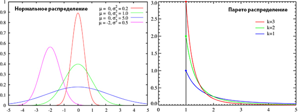
And ... suddenly, and ... the tests themselves for the normal distribution on the plotly are not correct? Looking ahead to say - everything is in order. I have generated two types of random samples - Gaussian and Pareto; These arrays are sequentially sent to plot.ly. We are testing. The nature of the distributions is very different and it is obvious that Pareto sampling does not have to pass the “normality” test.
Test code:
The processing results can be viewed in your profile at plot.ly/organize/home
So, here are some results of the Shapiro-Wilk tests:
For Pareto distribution
First test

Second test

For normal (Gaussian) distribution
First test

Second test

So, the test algorithm works correctly. However, the tips for using the test are not quite correct, to say the least. The moral of the following: beware! Near the correctly written tool does not always lie correctly written instructions!
Let us proceed to testing the movement of financial instruments for normality (Gauss) distribution using the plotly library. I obtained the following results:
The rest of the financial instruments have a similar picture. Therefore, we exclude the assumption that the distribution of the considered financial instruments is normal in motion. The test code itself:
Since we cannot rely on the normal (Gaussian) distribution - therefore, when calculating the correlations, it is necessary to choose a nonparametric tool, namely the Spearman correlation coefficient (Spearman rank correlation coefficient) . Once you have decided on the type of correlation, you can go directly to its calculations:
We get a file with correlations for the current paper (of the type corr_A.csv) and the previous period for other securities (B, C, D, there are only 90), for this we delete the first line with empty values in the file of the type securities_A.csv; We calculate the correlations of other securities in relation to the current one. Sort a column of correlations and naming to them. Save the correlation column for the current security as a separate DataFrame.

Alternately, each of the files with correlations of the type corr_A.csv is “merged” into one common file - _quotes_data_end.csv .csv. The lines in this file are impersonal. One can observe only the values of sorted correlations.

According to the data obtained _quotes_data_end.csv we build a graph:

The level of correlation even in the extreme regions is not high. The bulk of the correlation values is in the range of -0.15; 0.15. There are no such securities as such that “conducted” any other financial instruments within the period under review (7.5 months) and on this timeframe (“watch”). Let me remind you that we have at our disposal data on 91 securities. But ... if you try to process the same "watch" for a shorter period? For a sample of 1 month duration, we obtain the following graph:

Reducing the timeframe and reducing the size of the samples under consideration yields higher correlations. The myth of “locomotive” movements (when one paper “pulls” behind itself another, or acts as a “counterweight”) ... turns into reality. This effect is observed as the sample size decreases . However, as the flip side of the coin - an increase in the values of correlations at the same time, is accompanied by their increasingly unstable behavior . Paper from the "locomotive" can turn into a "slave" in a relatively short period of time. We can state that the methods of data processing were covered by us, the answers to the above questions were received.
What is the nature of the dynamics of changes in correlations; How does this happen and how is it accompanied? But ... this is a topic to continue.
Thanks for attention!
One of the legends of traders is the concept of "locomotive". It can be described as follows: there are “lead” papers and there are “follower” papers. If we believe in the existence of such a pattern, then we can “predict” the future movements of a financial instrument along the movement of “locomotives” (“leading” securities). Is it so? Is there a reason for this?
We formulate the problem. There are financial instruments: A, B, C, D; there is a time characteristic - t. Are there any links between the movements of these tools:
A t and B t-1 ; A t and C t-1 ; A t and D t-1
B t and C t-1 ; B t and D t-1 ; B t and A t-1
C t and D t-1 ; C t and A t-1 ; C t and B t-1
D t and A t-1 ; D t and B t-1 ; D t and B t-1
')
How to get data for the study of this issue? How strong, stable are the links mentioned? How can they be measured? What tools?
We first note that today there are a significant number of predictive models. Some sources say that their number has exceeded one hundred . By the way - the main joke of reality is that ... the more complex the model, the harder the interpretation, the understanding of each individual component of this model itself. I emphasize that the purpose of this article is to answer the above questions , and not to use one of the existing forecasting models.The pandas package is a powerful data analysis tool that has a rich arsenal of tools. We use its capabilities to study the questions raised by us.
Previously, we get quotes from the server of the company "FINAM". We will take the "watch" for the period from 01/01/2017 to 13/07/2017 . By slightly modifying the function mentioned here , we get:
# -*- coding: utf-8 -*- """ @author: optimusqp """ import os import urllib import pandas as pd import time import codecs from datetime import datetime, date from pandas.io.common import EmptyDataError e='.csv'; p='7'; yf='2017'; yt='2017'; month_start='01'; day_start='01'; month_end='07'; day_end='13'; year_start=yf[2:]; year_end=yt[2:]; mf=(int(month_start.replace('0','')))-1; mt=(int(month_end.replace('0','')))-1; df=(int(day_start.replace('0',''))); dt=(int(day_end.replace('0',''))); dtf='1'; tmf='1'; MSOR='1'; mstimever='0' sep='1'; sep2='1'; datf='5'; at='1'; def quotes_finam_optimusqp(data,year_start,month_start,day_start,year_end,month_end,day_end,e,df,mf,yf,dt,mt,yt,p,dtf,tmf,MSOR,mstimever,sep,sep2,datf,at): temp_name_file='id,company\n'; incrim=1; for index, row in data.iterrows(): page = urllib.urlopen('http://export.finam.ru/'+str(row['code'])+'_'+str(year_start)+str(month_start)+str(day_start)+'_'+str(year_end)+str(month_end)+str(day_end)+str(e)+'?market='+str(row['id_exchange_2'])+'&em='+str(row['em'])+'&code='+str(row['code'])+'&apply=0&df='+str(df)+'&mf='+str(mf)+'&yf='+str(yf)+'&from='+str(day_start)+'.'+str(month_start)+'.'+str(yf)+'&dt='+str(dt)+'&mt='+str(mt)+'&yt='+str(yt)+'&to='+str(day_end)+'.'+str(month_end)+'.'+str(yt)+'&p='+str(p)+'&f='+str(row['code'])+'_'+str(year_start)+str(month_start)+str(day_start)+'_'+str(year_end)+str(month_end)+str(day_end)+'&e='+str(e)+'&cn='+str(row['code'])+'&dtf='+str(dtf)+'&tmf='+str(tmf)+'&MSOR='+str(MSOR)+'&mstimever='+str(mstimever)+'&sep='+str(sep)+'&sep2='+str(sep2)+'&datf='+str(datf)+'&at='+str(at)) print('http://export.finam.ru/'+str(row['code'])+'_'+str(year_start)+str(month_start)+str(day_start)+'_'+str(year_end)+str(month_end)+str(day_end)+str(e)+'?market='+str(row['id_exchange_2'])+'&em='+str(row['em'])+'&code='+str(row['code'])+'&apply=0&df='+str(df)+'&mf='+str(mf)+'&yf='+str(yf)+'&from='+str(day_start)+'.'+str(month_start)+'.'+str(yf)+'&dt='+str(dt)+'&mt='+str(mt)+'&yt='+str(yt)+'&to='+str(day_end)+'.'+str(month_end)+'.'+str(yt)+'&p='+str(p)+'&f='+str(row['code'])+'_'+str(year_start)+str(month_start)+str(day_start)+'_'+str(year_end)+str(month_end)+str(day_end)+'&e='+str(e)+'&cn='+str(row['code'])+'&dtf='+str(dtf)+'&tmf='+str(tmf)+'&MSOR='+str(MSOR)+'&mstimever='+str(mstimever)+'&sep='+str(sep)+'&sep2='+str(sep2)+'&datf='+str(datf)+'&at='+str(at)) print('code: '+str(row['code'])) # . # - file = codecs.open(str(row['code'])+"_"+"0"+".csv", "w", "utf-8") content = page.read() file.write(content) file.close() temp_name_file = temp_name_file + (str(incrim) + "," + str(row['code'])+"\n") incrim+=1 time.sleep(2) # code , # - . write_file = "name_file_data.csv" with open(write_file, "w") as output: for line in temp_name_file: output.write(line) # quotes_finam_optimusqp # function_parameters.csv #___http://optimusqp.ru/articles/articles_1/function_parameters.csv data_all = pd.read_csv('function_parameters.csv', index_col='id') # , # id_exchange_2 == 1, .. data = data_all[data_all['id_exchange_2']==1] quotes_finam_optimusqp(data,year_start,month_start,day_start,year_end,month_end,day_end,e,df,mf,yf,dt,mt,yt,p,dtf,tmf,MSOR,mstimever,sep,sep2,datf,at) As a result, we have a list of files of type A_0.csv:
Next, we determine the movements of financial instruments A t -A t-1 , remove the columns OPEN, HIGH, LOW, VOL, form a single column DATETIME. We will eliminate those financial instruments that have too little data for analysis (they are traded recently, unstable or have low liquidity).
# , ? # - . name_file_data = pd.read_csv('name_file_data.csv', index_col='id') incrim=1; # how_work_days - , # , # temp_string_in_file='id,how_work_days\n'; for index, row1 in name_file_data.iterrows(): how_string_in_file = 0 # , name_file=row1['company']+"_"+"0"+".csv" # ? if os.path.exists(name_file): folder_size = os.path.getsize(name_file) # - , if folder_size>0: temp_quotes_data=pd.read_csv(name_file, delimiter=',') # , EmptyDataError # try: # (CLOSE); # quotes_data = temp_quotes_data.drop(['<OPEN>', '<HIGH>', '<LOW>', '<VOL>'], axis=1) # - how_string_in_file = len(quotes_data.index) # 1 100, # ; if how_string_in_file>1100: # days_data.csv, # # temp_string_in_file = temp_string_in_file + (str(incrim) + "," + str(how_string_in_file)+"\n") incrim+=1 quotes_data['DATE_str']=quotes_data['<DATE>'].astype(basestring) quotes_data['TIME_str']=quotes_data['<TIME>'].astype(basestring) #"" DATETIME quotes_data['DATETIME'] = quotes_data.apply(lambda x:'%s%s' % (x['DATE_str'],x['TIME_str']),axis=1) quotes_data = quotes_data.drop(['<DATE>','<TIME>','DATE_str','TIME_str'], axis=1) quotes_data['DATETIME'].apply(lambda d: datetime.strptime(d, '%Y%m%d%H%M%S')) quotes_data [row1['company']] = quotes_data['<CLOSE>'] - quotes_data['<CLOSE>'].shift(1) quotes_data = quotes_data.drop(['<CLOSE>'], axis=1) quotes_data.to_csv(row1['company']+"_"+"1"+".csv", sep=',', encoding='utf-8') os.unlink(row1['company']+"_"+"0"+".csv") else: os.unlink(row1['company']+"_"+"0"+".csv") except pd.io.common.EmptyDataError: os.unlink(row1['company']+"_"+"0"+".csv") else: os.unlink(row1['company']+"_"+"0"+".csv") else: continue write_file = "days_data.csv" with open(write_file, "w") as output: for line in temp_string_in_file: output.write(line) As a result, we get a list of files of type A_1.csv. Total 91 files:
We merge all movements of all financial instruments into one file securities.csv by deleting the first empty line.
import glob allFiles = glob.glob("*_1.csv") frame = pd.DataFrame() list_ = [] for file_ in allFiles: df = pd.read_csv(file_,index_col=None, header=0) list_.append(df) dfff = reduce(lambda df1,df2: pd.merge(df1,df2,on='DATETIME'), list_) quotes_data = dfff.drop(['Unnamed: 0_x', 'Unnamed: 0_y', 'Unnamed: 0'], axis=1) quotes_data.to_csv("securities.csv", sep=',', encoding='utf-8') quotes_data = quotes_data.drop(['DATETIME'], axis=1) number_columns=len(quotes_data.columns) columns_name_0 = quotes_data.columns columns_name_1 = quotes_data.columns At this stage, there is a rather interesting operation of merging records by the DATETIME column (pd.merge). This merger procedure discards those dates on which at least one of the 91 securities did not trade. That is, the union is based on the complete elimination of empty data. As a result:
In the file securities.csv , operating with data in a cycle, we shift all lines except the current one. Thus, on the contrary A t are the values B t-1 , C t-1 , D t-1 .
incrim=0 quotes_data_w=quotes_data.shift(1) for column in columns_name_0: quotes_data_w[column]=quotes_data_w[column].shift(-1) quotes_data_w.to_csv("securities_"+column+".csv", sep=',', encoding='utf-8') # quotes_data_w[column]=quotes_data_w[column].shift(1) incrim+=1 The data will look like this:
And yes, you need to delete the first row with empty data. Now you can build correlations between columns. They will then reveal the existence or absence of papers, “locomotives” ... or they will make it possible to make sure that “locomotives” are nothing more than a myth.
The fact of the absence of a normal (Gaussian) distribution in the movement of financial instruments is mentioned relatively recently. Nevertheless, the majority of financial models are based on his assumption. Is the Gaussian distribution present in our data? The question is not idle, since the existence of normality will allow the use of the Pearson correlation, and the absence will oblige the use of a nonparametric form of correlation. With this question we turn to plotly's wonderful service.
What is interesting this service? Firstly, the ability to graphically interpret the data. Secondly, a set of statistical test methods; in particular, the possibility of conducting tests for the conformity of the sample to the normal (Gaussian) distribution. We will use the following tests: the Shapiro-Wilk criterion (Shapiro-Wilk), the Kolmogorov-Smirnov criterion (Kolmogorov-Smirnov), see the rules of work here .The service related to plotly is worthy of the highest praise. Tutorial on setting up plotly on Linux can be viewed on plot.ly, and under Windows, for example, here . But there are plotly and weirdness. And the question here is nothing more than a description of the logic of the test. In the examples for the application table is given:
The developer gives the following comment:
Since our p-value is less than our test status, the numerical hypothesis at the 0.05 significance level.
Transfer:
Since our p-value is much smaller than our test statistics, we have good evidence that we do not reject the null hypothesis at the 0.05 significance level.
Thus, according to this recommendation, we are not entitled to abandon the hypothesis of normal distribution for the sample under consideration! But ... this advice is not correct .
So, remember - what is p-value? This value is necessary for testing statistical hypotheses. It can be understood as the probability of error if we reject the null hypothesis. Under the null hypothesis in the Shapiro-Wilk criterion H 0 , I recall, it means that "the random variable X is distributed normally." If we reject H 0 for an extremely small p-value (close to zero), then we will not be mistaken. We are not mistaken in eliminating the assumption of normal distribution. In general, the level of significance in the plotly tests for normality is 0.05, and acceptance or non-acceptance of the null hypothesis should be based on the comparison of this value to the p-value . Exceeding the threshold of the significance level by the p-value indicates that the hypothesis that the distribution of the test sample is normal cannot be rejected.
And ... suddenly, and ... the tests themselves for the normal distribution on the plotly are not correct? Looking ahead to say - everything is in order. I have generated two types of random samples - Gaussian and Pareto; These arrays are sequentially sent to plot.ly. We are testing. The nature of the distributions is very different and it is obvious that Pareto sampling does not have to pass the “normality” test.
Test code:
import pandas as pd import matplotlib.pyplot as plt import plotly.plotly as py import plotly.graph_objs as go from plotly.tools import FigureFactory as FF import numpy as np from scipy import stats, optimize, interpolate def Normality_Test(L): x = L shapiro_results = scipy.stats.shapiro(x) matrix_sw = [ ['', 'DF', 'Test Statistic', 'p-value'], ['Sample Data', len(x) - 1, shapiro_results[0], shapiro_results[1]] ] shapiro_table = FF.create_table(matrix_sw, index=True) py.iplot(shapiro_table, filename='pareto_file') #py.iplot(shapiro_table, filename='normal_file') #L =np.random.normal(115.0, 10, 860) L =np.random.pareto(3,50) Normality_Test(L) The processing results can be viewed in your profile at plot.ly/organize/home
So, here are some results of the Shapiro-Wilk tests:
For Pareto distribution
First test
Second test
For normal (Gaussian) distribution
First test
Second test
So, the test algorithm works correctly. However, the tips for using the test are not quite correct, to say the least. The moral of the following: beware! Near the correctly written tool does not always lie correctly written instructions!
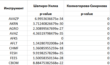
Let us proceed to testing the movement of financial instruments for normality (Gauss) distribution using the plotly library. I obtained the following results:
The rest of the financial instruments have a similar picture. Therefore, we exclude the assumption that the distribution of the considered financial instruments is normal in motion. The test code itself:
allFiles = glob.glob("*_1.csv") def Shapiro(df,temp_header): df=df.drop(df.index[0]) x = df[temp_header].tolist() shapiro_results = scipy.stats.shapiro(x) matrix_sw = [ ['', 'DF', 'Test Statistic', 'p-value'], ['Sample Data', len(x) - 1, shapiro_results[0], shapiro_results[1]] ] shapiro_table = FF.create_table(matrix_sw, index=True) py.iplot(shapiro_table, filename='shapiro-table_'+temp_header) def Kolmogorov_Smirnov(df,temp_header): df=df.drop(df.index[0]) x = df[temp_header].tolist() ks_results = scipy.stats.kstest(x, cdf='norm') matrix_ks = [ ['', 'DF', 'Test Statistic', 'p-value'], ['Sample Data', len(x) - 1, ks_results[0], ks_results[1]] ] ks_table = FF.create_table(matrix_ks, index=True) py.iplot(ks_table, filename='ks-table_'+temp_header) frame = pd.DataFrame() list_ = [] for file_ in allFiles: df = pd.read_csv(file_,index_col=None, header=0) print(file_) columns = df.columns temp_header = columns[2] Shapiro(df,temp_header) time.sleep(3) Kolmogorov_Smirnov(df,temp_header) time.sleep(3) Since we cannot rely on the normal (Gaussian) distribution - therefore, when calculating the correlations, it is necessary to choose a nonparametric tool, namely the Spearman correlation coefficient (Spearman rank correlation coefficient) . Once you have decided on the type of correlation, you can go directly to its calculations:
incrim=0 for column0 in columns_name_1: df000 = pd.read_csv('securities_'+column0+".csv",index_col=None, header=0) # df000=df000.drop(df000.index[0]) df000 = df000.drop(['Unnamed: 0'], axis=1) # # corr_spr=df000.corr('spearman') # # corr_spr=corr_spr.sort_values([column0], ascending=False) # DataFrame corr_spr_temp=corr_spr[column0] corr_spr_temp.to_csv("corr_"+column0+".csv", sep=',', encoding='utf-8') incrim+=1 We get a file with correlations for the current paper (of the type corr_A.csv) and the previous period for other securities (B, C, D, there are only 90), for this we delete the first line with empty values in the file of the type securities_A.csv; We calculate the correlations of other securities in relation to the current one. Sort a column of correlations and naming to them. Save the correlation column for the current security as a separate DataFrame.
Alternately, each of the files with correlations of the type corr_A.csv is “merged” into one common file - _quotes_data_end.csv .csv. The lines in this file are impersonal. One can observe only the values of sorted correlations.
incrim=0 all_corr_Files = glob.glob("corr_*.csv") list_corr = [] quotes_data_end = pd.DataFrame() for file_corr in all_corr_Files: df_corr = pd.read_csv(file_corr,index_col=None, header=0) columns_corr = df_corr.columns temp_header = columns_corr[0] quotes_data_end[str(temp_header)]=df_corr.iloc[:,1] incrim+=1 quotes_data_end.to_csv("_quotes_data_end.csv", sep=',', encoding='utf-8') plt.figure(); quotes_data_end.plot(); According to the data obtained _quotes_data_end.csv we build a graph:
The level of correlation even in the extreme regions is not high. The bulk of the correlation values is in the range of -0.15; 0.15. There are no such securities as such that “conducted” any other financial instruments within the period under review (7.5 months) and on this timeframe (“watch”). Let me remind you that we have at our disposal data on 91 securities. But ... if you try to process the same "watch" for a shorter period? For a sample of 1 month duration, we obtain the following graph:
Reducing the timeframe and reducing the size of the samples under consideration yields higher correlations. The myth of “locomotive” movements (when one paper “pulls” behind itself another, or acts as a “counterweight”) ... turns into reality. This effect is observed as the sample size decreases . However, as the flip side of the coin - an increase in the values of correlations at the same time, is accompanied by their increasingly unstable behavior . Paper from the "locomotive" can turn into a "slave" in a relatively short period of time. We can state that the methods of data processing were covered by us, the answers to the above questions were received.
What is the nature of the dynamics of changes in correlations; How does this happen and how is it accompanied? But ... this is a topic to continue.
Thanks for attention!
Source: https://habr.com/ru/post/334288/
All Articles