Non-standard clustering, part 3: techniques and metrics for time series clustering
Part One - Affinity Propagation
Part Two - DBSCAN
Part Three - Time Series Clustering
Part Four - Self-Organizing Maps (SOM)
Part Five - Growing Neural Gas (GNG)
While other specialists in machine learning and data analysis are figuring out how to tie more layers to the neural network so that it plays Mario even better, let's turn to something more mundane and applicable in practice.
Clustering time series is a thankless job. Even when grouping static data, dubious results are often obtained, let alone information that is scattered over time. However, you can not ignore the task, just because it is difficult. Let's try to figure out how to squeeze out a little sense from the rows without tags. This article discusses subtypes of time series clustering, general techniques, and popular measures of row spacing. The article is intended for readers who have already dealt with sequences in data science: the basic things (trend, ARMA / ARIMA, spectral analysis) will not be discussed.
Hereinafter P , Q , R - time series with time counts t 1 d o t s t n and levels x 1 d o t s x n , y 1 d o t s y n and z 1 d o t s z n respectively. Time Series Values - x i , y i , z i - one-dimensional real variables. Variable t is considered time, but the mathematical abstractions discussed below are generally applicable to spatial series (an expanded curve), to series of symbols and sequences of other types (say, the graph of the emotional color of the text). D ( P , Q ) - a function that measures how much P differs from Q . It’s easiest to think of it as a distance from P before Q However, it should be remembered that it does not always correspond to the mathematical definition of a metric.
')
When working with time series, there are many typical data science difficulties: high dimensionality of input data, missing data, correlated noise. However, in the task of clustering sequences there are a couple of additional difficulties. First, in the ranks there can be a different number of readings. Secondly, when working with sequential data, we have more degrees of freedom in determining how one element is similar to another. The point here is not only in the number of variables in the dataset instance; The way data changes over time also contributes. This is an obvious, but important point: we can independently transform or renumber the values of instances of static data, but this will not work with sequences. Therefore, metrics and algorithms must take into account local data dependency.

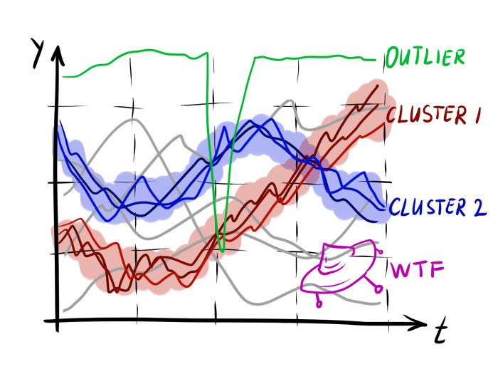
In addition, when clustering rows, the semantics of the data makes a stronger contribution. For example, how to distribute 8 graphs in the picture into groups?
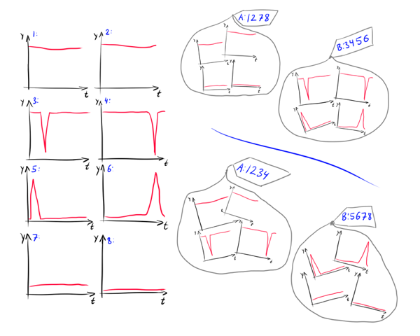
What is more important for a researcher? Average level y or the presence of jumps? If myself y then the first partition 1234/5678 is better suited; if it changes, then the best one will be 1278/3456. Moreover, is it important when exactly the jump occurs? Maybe we should break the group 3456 into subgroups 34 and 56? Depending on what exactly is y , these questions can be given different answers.
Therefore, in connection with the possible semantic differences of the data, it is useful to distinguish several types of similarity that may occur in practical problems [1]

A clear understanding of which type of similarity is characteristic of your task is an integral part in creating meaningful clusters.
A large amount of input data suggests feature engineering. The best way to cluster time series is to cluster them NOT as time series. If the specifics of the task allows you to convert samples to fixed-size data, you should use this opportunity. Immediately disappears a whole group of problems.

If you cannot get rid of the time dependence at all, then you should try to at least simplify the series or transfer it to another area:
The above global characteristics will allow you to divide the rows into groups of similar structure. When this alone does not give meaningful results, you should select the appropriate metric on the sequence space. To highlight clear patterns in the information, you need to construct a good proximity function, but in order to do this, you must already have some idea of the existing dataset, so do not dwell on any one of the options presented below.
Alas, I did not find adapted clustering algorithms for sequential data, which would be interesting to tell. Maybe I don’t know something, but several evenings spent at ArXiv and IEEE did not bring me any insights. It seems that scientists are limited only to the study of new metrics for comparing time series, but are not eager to invent specialized algorithms. The whole trick occurs at the stage of calculating the distance matrix, and the division into groups itself is carried out by good old algorithms for static data: k-means derivatives, DBSCAN, Affinity propagation, trivial hierarchical clustering, and others. There are a few that can be looked at [10] [11] [12] [13], but not that their results are much better than the old methods.
K-means gives decent results less often than in the case of static data. Some researchers have succeeded in successfully applying DBSCAN, but for him it is very nontrivial to find good parameters: the main area of its application is by no means time series. The last two candidates in the list look much more interesting, hierarchical clustering is used most often [14] [15] [16]. Modern approaches also predispose the computation and combination of several distance matrices using different metrics.
Summary.You have a pack of time series in your hands, and you don’t know what to do with it?
First of all, check whether there are any missing values or explicit counting of emissions. Then try to output part of dataset and see
Try to collect statistical data across the rows and cluster them; k-means derivatives are appropriate here. If this is not enough, see if any of the variables have a clearly bimodal distribution (in particular, a trend) - this may help in understanding the dataset.
Calculate the distance matrix using DTW or several TWED approaches with different parameters. Output the result of the hierarchical clustering algorithm. Try to formulate a hypothesis about the form of dataset. Change the metric according to the situation, or combine several metrics. Repeat.
And most importantly: try to get knowledge of what the meanings of these sequences really mean. This can radically affect the choice of metrics.
Yeah ... not that this algorithm is very different from any rough data processing. What to do, clustering the time series is hard work, and too much depends on specific data. I hope my article will help at least a little if you have to deal with it. In the end, even a small increase in the quality of computer data processing can mean for a human specialist the difference between "nothing is clear" and "it seems like a pattern can be found."
[1] Saeed Aghabozorgi, Ali Seyed Shirkhorshidi, Teh Ying Wah - Time-series clustering - a Decade Review
[2] Konstantinos Kalpakis, Dhiral Gada, and Vasundhara Puttagunta - Distance Measures for Effective Clustering of ARIMA Time-Series.
[3] Subsequence Time Series (STS) Clustering Techniques for Meaningful Pattern Discovery
[4] Li Junkui, Wang Yuanzhen, Li Xinping - LB HUST: A Symmetrical Boundary Distance for Clustering Time Series
[5] Joan Serria, Joseph Arcos - A Competitive Measure
[6] PF Marteau - Time Warp
[7] Gustavo EAPA Batista, Xiaoyue Wang, Eamonn J. Keogh - A Complexity-Invariant Distance Measure for Time Series
[8] Vo Thanh Vinh, Duong Tuan Anh - Compression Rate
[9] Dinkar Sitaram, Aditya Dalwani, Anish Narang, Madhura Das, Auradkar
[10] John Paparrizos, Luis Gravano - K-Shape: Efficient and Accurate Clustering of Time Series // Fast and Accurate Time-Series Clustering
[11] Leonardo N. Ferreiraa, Liang Zhaob - Time Series Clustering via Community Detection in Networks
[12] Zhibo Zhu, Qinke Peng, Xinyu Guan - A Time Series Clustering Method Based on Hypergraph Partitioning
[13] Shan Jicheng, Liu Weike - Clustering Algorithm for Time Series Based on Peak Interval
[14] Sangeeta Rani - Modified Clustering Algorithm for Time Series Data
[15] Pedro Pereira Rodrigues, Joao Gama, Joao Pedro Pedroso - Hierarchical Clustering of Time Series Data Streams
[16] Financial Time Series based on Agglomerative Hierarchical Clustering
[17] Goctug T. Cinar and Jose C. Principe - Hierarchical Linear Dynamic System
Part Two - DBSCAN
Part Three - Time Series Clustering
Part Four - Self-Organizing Maps (SOM)
Part Five - Growing Neural Gas (GNG)
While other specialists in machine learning and data analysis are figuring out how to tie more layers to the neural network so that it plays Mario even better, let's turn to something more mundane and applicable in practice.
Clustering time series is a thankless job. Even when grouping static data, dubious results are often obtained, let alone information that is scattered over time. However, you can not ignore the task, just because it is difficult. Let's try to figure out how to squeeze out a little sense from the rows without tags. This article discusses subtypes of time series clustering, general techniques, and popular measures of row spacing. The article is intended for readers who have already dealt with sequences in data science: the basic things (trend, ARMA / ARIMA, spectral analysis) will not be discussed.
Hereinafter P , Q , R - time series with time counts t 1 d o t s t n and levels x 1 d o t s x n , y 1 d o t s y n and z 1 d o t s z n respectively. Time Series Values - x i , y i , z i - one-dimensional real variables. Variable t is considered time, but the mathematical abstractions discussed below are generally applicable to spatial series (an expanded curve), to series of symbols and sequences of other types (say, the graph of the emotional color of the text). D ( P , Q ) - a function that measures how much P differs from Q . It’s easiest to think of it as a distance from P before Q However, it should be remembered that it does not always correspond to the mathematical definition of a metric.
')
Time series “similarity” subtypes
When working with time series, there are many typical data science difficulties: high dimensionality of input data, missing data, correlated noise. However, in the task of clustering sequences there are a couple of additional difficulties. First, in the ranks there can be a different number of readings. Secondly, when working with sequential data, we have more degrees of freedom in determining how one element is similar to another. The point here is not only in the number of variables in the dataset instance; The way data changes over time also contributes. This is an obvious, but important point: we can independently transform or renumber the values of instances of static data, but this will not work with sequences. Therefore, metrics and algorithms must take into account local data dependency.
In addition, when clustering rows, the semantics of the data makes a stronger contribution. For example, how to distribute 8 graphs in the picture into groups?
What is more important for a researcher? Average level y or the presence of jumps? If myself y then the first partition 1234/5678 is better suited; if it changes, then the best one will be 1278/3456. Moreover, is it important when exactly the jump occurs? Maybe we should break the group 3456 into subgroups 34 and 56? Depending on what exactly is y , these questions can be given different answers.
Therefore, in connection with the possible semantic differences of the data, it is useful to distinguish several types of similarity that may occur in practical problems [1]
- Rows are similar in time. The easiest type of similarity. We are looking for series where the singular points and intervals of increasing exactly or almost exactly match each other in time. In this case, it is not necessary that the values of the extremes and the slopes of the curves coincide exactly with each other, if only they are close on average. This type of similarity arises, for example, in market analysis tasks, when we want to discover clusters of companies whose shares fall and grow together. In the figure below, graphs 1 and 2 are similar in time.
- The rows are similar in shape. We are looking for rows with the same characteristics, but not overlapping each other. They can be either just separated in time, or stretched or somehow transformed. This type of similarity occurs, for example, when clustering sound samples - it is impossible to pronounce the same phrase at exactly the same pace. Figures 3 and 4 in the figure are similar in shape.
- Rows similar in structure. Search for sequences with the same laws of change; as global - periodicity (5 and 6), trend (7 and 8) - and local, for example, how many times a certain pattern occurs in a sequence.
A clear understanding of which type of similarity is characteristic of your task is an integral part in creating meaningful clusters.
Receptions for the presentation of data
A large amount of input data suggests feature engineering. The best way to cluster time series is to cluster them NOT as time series. If the specifics of the task allows you to convert samples to fixed-size data, you should use this opportunity. Immediately disappears a whole group of problems.
- The best case is when a mathematical model is known in advance that the data meets (for example, it is given that the sequence is the sum of a finite set of functions and noise, or the generating model is known). Then it is worth translating sequences into the model parameter space, and clustering already in it [17]. Unfortunately, such happiness rarely falls.
- It is worth seeing how a good result can be obtained by collecting simple statistics on a dataset:
- minimum, maximum, average and median elements (after smoothing)
- number of peaks and valleys
- element dispersion
- the area under the schedule (before normalization and subtraction of the average, if you want to hold them)
- sum of squares of the derivative
- trend indicator
- ARIMA coefficients, if applicable [2]
- the number of intersections of marks in the 25th, 50th, 75th percentile, the intersection of the average and zero
Even if the clustering of statistical reports by series alone does not give good results, try attaching these global parameters to the original data. This will help to divide the rows with similarity in structure. - You can try the bag of features approach. Characteristic forms can either be set and found manually, or determined automatically by the auto-encoder. In general, approaches based on clustering of subsequences have recently experienced a rise and fall in popularity. It has been shown that too often they produce meaningless results. But if you are sure that the rows from dataset have some characteristic subsequences, go for it [3].
- If you do not want to mess around with the frequency domain, but nevertheless, the idea of clustering series based on cyclical features seems sensible, try converting the series into an autocorrelation region and group the data already in it.
If you cannot get rid of the time dependence at all, then you should try to at least simplify the series or transfer it to another area:
- If the data is noisy or has a very large dimension, then it is worth it to thin it. Use your favorite method of interval interpolation (the simplest is linear approximation, Piecewise Linear Approximation, PLA, or intervalline interpolation by splines) or the algorithm for finding special points (Perceptually Important Points, PIP).
- In the case of very noisy data, it is also possible to construct the upper and lower envelope for each time sequence, and cluster the pairs that have already been obtained. Instead of one row, it turns out two, which does not look like a simplification at all, but being applied for its intended purpose, this approach makes the data more understandable for both humans and computers [4].
- In bioinformatics and processing character sequences, it is often useful to apply character encoding (Symbolic Approximation, SAX) to a series.
- Frequency indicators. Discrete Fourier transform, wavelet transform, cosine transform. This is not the best option, as we move from one sequence to another, often even more incomprehensible, but sometimes it can help. By the way, if the Fourier transform helps so well, it may be worth using other digital signal processing tools.
Metrics
The above global characteristics will allow you to divide the rows into groups of similar structure. When this alone does not give meaningful results, you should select the appropriate metric on the sequence space. To highlight clear patterns in the information, you need to construct a good proximity function, but in order to do this, you must already have some idea of the existing dataset, so do not dwell on any one of the options presented below.
- Euclidean or L 1 -distance. These favorite metrics of all work only in the case of finding rows of similar time. Yes, and in this case, they can produce questionable results, if the sequence is long or noisy. But once a year and shuffle sort shoots.
Trivial improvement L 1 / L 2 -metrics is its upper limit, soft or hard: creating the maximum threshold for the contribution of the difference between sample levels with one t . Use it if you expect single count emissions to spoil an array of distances.
An example of a hard limit:hatL2(xi,yi)= begincasesL2(xi,yi),L2(xi,yi)< sigma sigma,L2(xi,yi) geq sigma endcases
An example of a soft constraint (near zero, the function behaves like L2 but with a big difference between xi and yi goes to level):hatL2(xi,yi)= frac(xi−yi)21+(xi−yi)2
Hereinafter, if the metric cannot be directly applied to rows of different lengths, try either stretching the smaller row to a larger size, or stretching it through the larger one (in the manner of cross-correlation) and taking the shortest distance. - Minimum Jump Cost (Minimum Jump Cost, MJC) [5]. An interesting dissimilarity function that has a simple intuitive meaning. We set the graphics flush with each other, after which we move from left to right, jumping from one chart to the closest (in a sense) point of another and back. This imposes a restriction that you can only select points that are ahead in time. The length of the path and will be MJC.

Formal definition by the authors of the article:MJCXY= sumicimin
cimin= min(ctytx,cty+1tx, dotscty+Ntx)
cty+ Deltatx=( phi Delta)2+(xti−yty+ Delta)2
phi= beta frac4 sigma min(M,N)
Where phi - the cost of advancement in time, it is desirable to make it proportional sigma standard deviation of the distribution of levels in the sequences, and inversely proportional to the size of the compared series. beta - control parameter less than beta the more elastic the measure is. With beta=0 the jump will be made to the closest level, regardless of where it is located; at beta rightarrow infty a jump in essence will always be made to a point with ti+1 .
It is easy to see that the function is asymmetrical, but this can be corrected if we set MJC(P,Q) = min(MJCXY(P,Q),MJCXY(Q,P)) or MJC(P,Q) = fracMJCXY(P,Q)+MJCXY(Q,P)2
beta it makes sense to select in such a way as to avoid the situation when the nearest cimin there is a point somewhere at the end of the series, and the algorithm “slips” the entire series (see figure). The specific values depend on the amplitude of the values. y and t .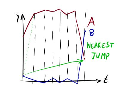
Actually, the insidious "in a certain sense" a couple of paragraphs above refers specifically to phi : cty+ Deltatx turned skewed. In fact, it is not necessary to dwell on simply re-weighting the Euclidean metric. Why not replace ( phi Delta)2 on ( phi Delta)4 with correction beta ? (Think how it will affect the behavior MJC(P,Q) - task for the curious reader;))
MJC - the development of the idea of a Euclidean metric with an upper bound on the contribution of readings. If in hatL2 emissions make a fixed contribution, then the backstory of the series plays a role in MJC. In the simplest case, the penalty increases quadratically. Moreover, what level is considered an outlier for a given pair of rows is automatically determined. The full story is a bit more complicated, but it is not too much a distortion to summarize that the MJC “forgives” single emissions, but gives more importance than hatL2 if there are long, very different sections in the rows.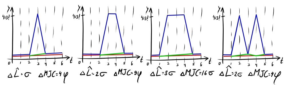
Use the MJC by default when it is known that the rows do not “break apart” in time, since most often the data is affected by white noise rather than grouped outliers. - Cross correlation This measure of proximity should be used when singular points and intervals in rows can be shifted in time from each other, but the shift is fixed - the internal distance between important elements is preserved. Characteristic points can appear and disappear, plus, compared time series can be of different duration. An excellent choice if it is known that the structure of sequences is not distorted in time (“hard” similarity in form). Also in this case, you can simply count L2 for each possible offset of one row relative to another.
Occasionally, cross-correlation is very helpful, but, as a rule, where the offset is, there is also a distortion. So much more used ... - Dynamic Timeline Transformation (Dynamic Time Warping, DTW).
It often happens that the characteristic parts of time series are not only separated from each other along the time axis, but also stretched or compressed. Then neither the Euclidean metric nor the cross-correlation gives significant results.
The DTW-algorithm builds a matrix of possible mappings of one row to another, given that the readings of the rows can either shift or change the level. The path in this matrix with the minimum value of the cost is DTW-distance. A similar principle is used in the Wagner-Fisher algorithm for finding the minimum editorial distance between lines.
The formal description of the algorithm can be read on Wikipedia, but I will try to go through the main points in a semi-formal way. Take two sequences P = \ {2, 6, 5, 3, 2 \} ; Q = \ {1,2,4,1,2 \} . They have a similar shape, but their peaks are offset from each other. Calculate the distance matrix d between each pair of levels. In this step, the usual is usually used. L1 or L2 . Then we will build a transformation matrix. D . We will fill it from left to right, top-down, according to the rule Di,j=di,j+ min(Di,j,Di−1,j,Di,j−1) . D1,1=d1,1 for the upper column and the left row of the part of the members in min not.
Build a path from DM,N at D1,1 each time moving into a cell with the smallest possible number. Every cell visited (i,j) will mean that with optimal transformation point j the first row is displayed on j -th second point. The cost of such a transformation consists of the difference between the levels of these points and the cost of the optimal transformation of all points to this pair. You can compare several points with one point, but we will only move to the left, up or (preferably) left-up, so that there is progress.
There are many such ways to build, but the best of them will be the one that minimizes frac sumKidi,jK where K is the path length, and di,j - value in the distance matrix.
DTW is a great feature for calculating time series differences, actually a baseline for comparison with other metrics. It is widely used as in problems of comparing segments of sound and when comparing sections of the genome. Feel free to use it when the rows should be similar in shape, but nothing is known about the maximum amount of shift or distortion. However, it also has flaws. First, it is long considered and / or requires additional memory, secondly, DTW does not always show an adequate distance when adding new characteristic points to a sequence. To make matters worse, it’s not so easy to estimate by eye as changing one of the rows will affect the way to D .
It is worth mentioning about the proximity function Edit Distance with Real Penalty (ERP) with similar behavior, but more condescendingly related to readings and emissions that cannot be compared. In addition, you can not ignore the side of Time Warp Edit Distance with Stiffness (TWED) [6]. The authors of this metric have developed a more general approach to describing proximity functions based on delete-match-insert operations (the Wagner-Fisher algorithm sends hello again), so DTW and ERP are special cases of TWED.
ERP and TWED - parametric; DTW - no. On the one hand, it is convenient, on the other hand, sometimes such infinite elasticity harms. There is a fast version of DTW, a version for sparse data, and a huge number of implementations of this algorithm. - Longest Common Distance (Longest Common Distance, LCD / Longest Common Subsequence, LCSS). LCSS is used in sequences where sample values are class labels, or where just a small number of levels. In the latter case, the LCSS can be modified to find the longest segment on which the difference in the values of the series is less than a certain threshold.
- Frechet discrete distance, it is also a concatenated distance. A semi-formal explanation is this: we will move point A in the sequence P, and point B in Q, perhaps unevenly. In such a case, the Fréchet distance between P and Q will be the minimum possible distance between A and B, with which both points can be drawn through the curves. Brrr ... better look at the example of a dog on a leash on Wikipedia. In our case Fr(P,Q)= maxi|xi−yi| but modifications are possible. It is suitable for rare cases when it is known that there are no counting of emissions in dataset, but there are rows of the same shape that are vertically offset from each other.
It is useful to compare the LCD and the Fréchet distance. If in the first case we take some maximum threshold and see which maximum sub-segment can be passed without exceeding it, then in the second we go through both sequences and see what minimum threshold we need for this. Both of these measures are used in tasks with similarity in time when some additional information is known. - Distance corrected for complexity (Complexity Invariant Distance, CID) [7]
Sometimes it is useful to add additional factors to the metric to help resolve contentious cases. For example, it happens that the rows P and Q coincide with each other throughout almost the entire length of time, but differ greatly at several points, and the row R does not at all look like the row P in shape, but is nevertheless close to it in average. As a rule, we would like to consider P and Q as more similar to each other.
As an additional factor, you can take the "complexity" of the sequence. If the curves P, Q and R have the same pairwise distance, but the curves P and Q, in addition, have the same “complexity”, then we will consider P and Q more similar.
“Complexity” can be measured differently, but do not forget that this parameter should be easily considered and have good interpretability. CID , , :CID(P,Q)=D(P,Q)×CF(P,Q)
CF(P,Q)=max(CE(P),CE(Q))min(CE(P),CE(Q))
CE(Q)=m∑i=1√(yi−yi−1)2+(ti−ti−1)2
Where D(P,Q) — ( ). — :CE(Q)=√m∑i=1(yi−yi−1)2

, «» — — , CID ( ≈2% ) . - (Compression Rate Distance, CRD)[8]
CRD, - D(P,Q) . , , Q , P . , , P and Q . , « » , — .∀ti←round[ti−minTmaxT−minT(2b−1)]+1
E(Q)=−∑tP(T=t)log2P(T=t)
DL(Q)=len(Q)×E(Q)
CR(P,Q)=DL(Q−P)min(DL(Q),DL(P))+ϵ
And finally:CRD(P,Q)=D(P,Q)×CR(P,Q)α
:ECRD(P,Q)=D(P,Q)×(1+CR(P,Q))α
Where alpha — CRD, ϵ . As D . ϵ=0.0001,α=2 and ϵ=0.0001,α=5 UCR Time Series Data Mining Site. , CRD , ( ≈4% ) CID ( ≈2% ). , + CRD - , DTW, , , . , CID: , CID .
CRD- , , y — . , CRD , P and Q . , , . 1 2 CRD, , . 3 4 CRD, , 1 2 . . , — . , CID , .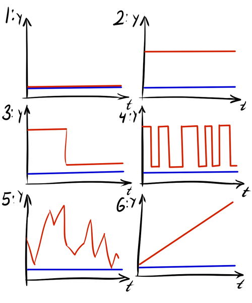
CRD , « » . , 5 6 , , . - [9]
, 1936 . , :D(P,Q)=√(x−y)TS−1(x−y)
S — . :D(P,Q)=√∑i(xi−yi)2σ2i
, , , . , , . , : — , — . .
, , , , . DTW-.
Conclusion
Alas, I did not find adapted clustering algorithms for sequential data, which would be interesting to tell. Maybe I don’t know something, but several evenings spent at ArXiv and IEEE did not bring me any insights. It seems that scientists are limited only to the study of new metrics for comparing time series, but are not eager to invent specialized algorithms. The whole trick occurs at the stage of calculating the distance matrix, and the division into groups itself is carried out by good old algorithms for static data: k-means derivatives, DBSCAN, Affinity propagation, trivial hierarchical clustering, and others. There are a few that can be looked at [10] [11] [12] [13], but not that their results are much better than the old methods.
K-means gives decent results less often than in the case of static data. Some researchers have succeeded in successfully applying DBSCAN, but for him it is very nontrivial to find good parameters: the main area of its application is by no means time series. The last two candidates in the list look much more interesting, hierarchical clustering is used most often [14] [15] [16]. Modern approaches also predispose the computation and combination of several distance matrices using different metrics.
Summary.You have a pack of time series in your hands, and you don’t know what to do with it?
First of all, check whether there are any missing values or explicit counting of emissions. Then try to output part of dataset and see
- are there any similar, but shifted in time relative to each other graphs
- are there any emissions, how systematically are they encountered
- are there any graphics with a pronounced periodicity
- Are there typical areas where the variance or rate of change of the rows is clearly different from other areas
Try to collect statistical data across the rows and cluster them; k-means derivatives are appropriate here. If this is not enough, see if any of the variables have a clearly bimodal distribution (in particular, a trend) - this may help in understanding the dataset.
Calculate the distance matrix using DTW or several TWED approaches with different parameters. Output the result of the hierarchical clustering algorithm. Try to formulate a hypothesis about the form of dataset. Change the metric according to the situation, or combine several metrics. Repeat.
And most importantly: try to get knowledge of what the meanings of these sequences really mean. This can radically affect the choice of metrics.
Yeah ... not that this algorithm is very different from any rough data processing. What to do, clustering the time series is hard work, and too much depends on specific data. I hope my article will help at least a little if you have to deal with it. In the end, even a small increase in the quality of computer data processing can mean for a human specialist the difference between "nothing is clear" and "it seems like a pattern can be found."
Sources
[1] Saeed Aghabozorgi, Ali Seyed Shirkhorshidi, Teh Ying Wah - Time-series clustering - a Decade Review
[2] Konstantinos Kalpakis, Dhiral Gada, and Vasundhara Puttagunta - Distance Measures for Effective Clustering of ARIMA Time-Series.
[3] Subsequence Time Series (STS) Clustering Techniques for Meaningful Pattern Discovery
[4] Li Junkui, Wang Yuanzhen, Li Xinping - LB HUST: A Symmetrical Boundary Distance for Clustering Time Series
[5] Joan Serria, Joseph Arcos - A Competitive Measure
[6] PF Marteau - Time Warp
[7] Gustavo EAPA Batista, Xiaoyue Wang, Eamonn J. Keogh - A Complexity-Invariant Distance Measure for Time Series
[8] Vo Thanh Vinh, Duong Tuan Anh - Compression Rate
[9] Dinkar Sitaram, Aditya Dalwani, Anish Narang, Madhura Das, Auradkar
[10] John Paparrizos, Luis Gravano - K-Shape: Efficient and Accurate Clustering of Time Series // Fast and Accurate Time-Series Clustering
[11] Leonardo N. Ferreiraa, Liang Zhaob - Time Series Clustering via Community Detection in Networks
[12] Zhibo Zhu, Qinke Peng, Xinyu Guan - A Time Series Clustering Method Based on Hypergraph Partitioning
[13] Shan Jicheng, Liu Weike - Clustering Algorithm for Time Series Based on Peak Interval
[14] Sangeeta Rani - Modified Clustering Algorithm for Time Series Data
[15] Pedro Pereira Rodrigues, Joao Gama, Joao Pedro Pedroso - Hierarchical Clustering of Time Series Data Streams
[16] Financial Time Series based on Agglomerative Hierarchical Clustering
[17] Goctug T. Cinar and Jose C. Principe - Hierarchical Linear Dynamic System
Source: https://habr.com/ru/post/334220/
All Articles