How to teach your neural network to generate poems
I beg you to stop dreaming me
I love you my bride
White frost on your eyelashes
Kiss on the body wordless
Once at school, it seemed to me that writing poetry was simple: you just need to arrange the words in the right order and select the right rhyme. Traces of these hallucinations (or illusions, I do not distinguish them) met you in the epigraph. Only this poem is, of course, not the result of my then creative work, but a product of a neural network trained on the same principle.
Rather, the neural network is needed only for the first stage - the arrangement of words in the correct order. The rules applied on top of the neural network predictions cope with rhyming. Want to know more about how we implemented it? Then welcome under cat.
Let's start with the language model. On Habré, I have met not too many articles about them - it would not be superfluous to recall what kind of beast it is.
')
Language models determine the likelihood of a sequence of words in this language:
  . Let us move from this terrible probability to the product of conditional probabilities of a word from an already read context:
 .
.
In life, these conditional probabilities show what word we expect to see next. Let us see, for example, the well-known words from Pushkin:
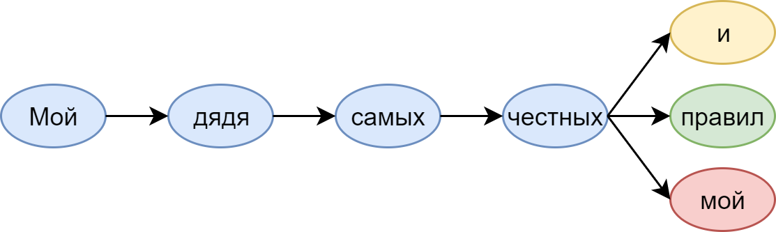
The language model that sits with us (in any case, with me) in my head suggests: after honest ones mine is unlikely to go again. And here, and, of course, the rules - very much so.
It seems the easiest way to build such a model is to use N-gram statistics. In this case, we approximate the probability - rejecting words that are too far away as they do not affect the probability of a given occurrence.
Such a model is easily implemented with the help of Counter on Python - and it turns out to be very heavy and not too variable. One of its most noticeable problems is the lack of statistics: most of the 5-gram words, including those permissible by the language, simply cannot be found in any large body.
To solve such a problem, Kneser – Ney or Katz's backing-off is usually used. For more information on N-gram smoothing methods, refer to Christopher Manning's famous book “Foundations of Statistical Natural Language Processing”.
I want to note that I called the 5-grams of words for a reason: it is them (with anti-aliasing, of course) that Google demonstrates in the article “One Billion Word Benchmark for Measuring Progress in Statistical Language Modeling” - and it shows results that are quite comparable to those of recurrent neural networks - which, in fact, will be discussed further.
Neural Network Language Models
The advantage of recurrent neural networks is the ability to use an infinitely long context. Together with each word arriving at the input of a recurrent cell, a vector appears in it representing the entire previous history — all the words processed to a given moment (the red arrow in the picture).
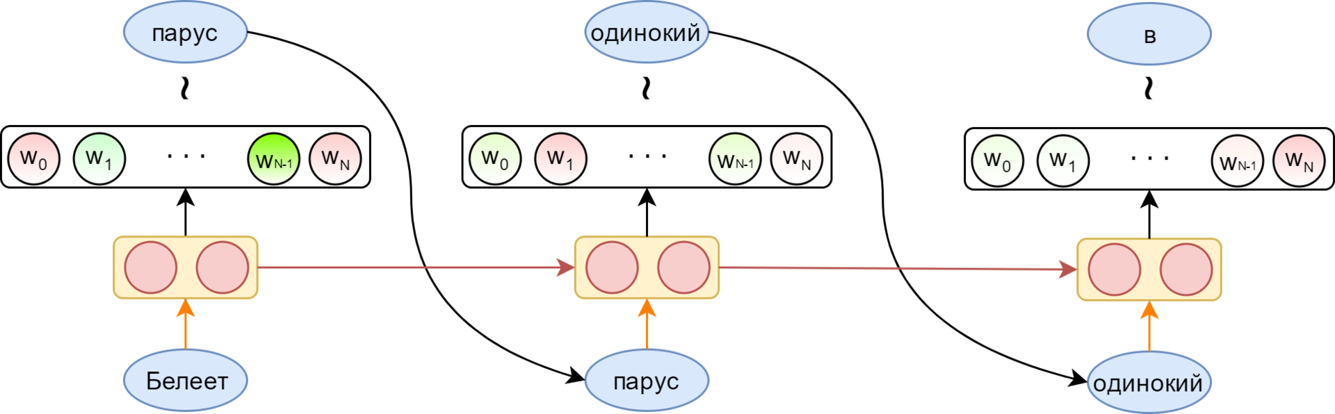
The possibility of using the context of unlimited length is, of course, only conditional. In practice, classic RNNs suffer from gradient damping - in fact, the inability to remember the context further than a few words. To combat this, special memory cells were invented. The most popular are LSTM and GRU. In the following, speaking of the recurrent layer, I will always mean LSTM.
The red arrow in the picture shows the display of the word in its embedding. The output layer (in the simplest case) is a fully connected layer with a size corresponding to the size of the dictionary, having softmax activation — to obtain a probability distribution for the vocabulary words. From this distribution, you can sample the next word (or just take the maximum possible).
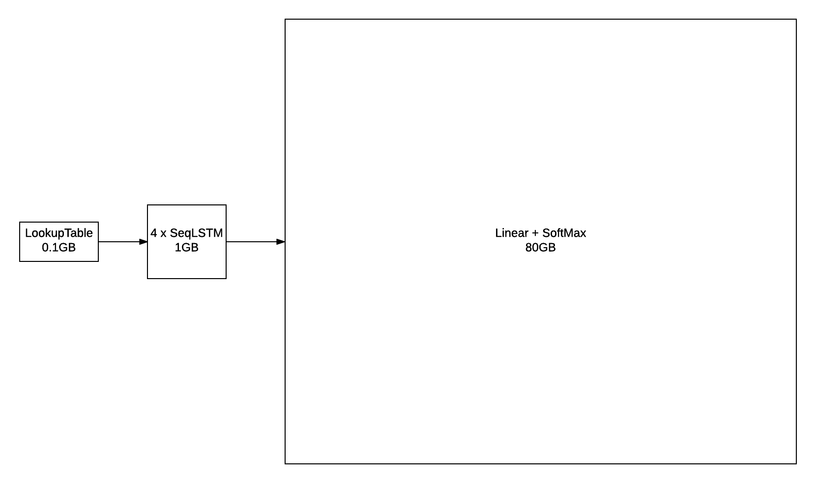
Already in the picture you can see a minus of such a layer: its size. With a dictionary of several hundred thousand words, he can easily stop getting on a video card, and his body requires huge corpus of texts. This is very clearly demonstrates the picture from the blog torch :
To combat this, a very large number of different techniques were invented. The most popular are hierarchical softmax and noise contrastive estimation. Details about these and other methods should be read in the excellent article Sebastian Ruder .
A more or less standard loss function, optimized for multi-class classification, is the cross-entropy loss function. In general, cross-entropy between vectors and the predicted vector
  recorded as
  . It shows the proximity of the distributions given by and .
When calculating cross-entropy for multi-class classification - this is the probability
  first class, and - a vector obtained with one-hot-encoding (i.e., a bit vector in which a single unit is at the position corresponding to the class number). Then
  with some
  .
.
Cross-entropy loss of the whole sentence are obtained by averaging the values over all words. They can be written as:
  . It can be seen that this expression corresponds to what we want to achieve: the probability of a real sentence from the language should be as high as possible.
In addition, perplexity is a metric specific to language modeling:
 .
.
To understand its meaning, let's look at a model that predicts words from the dictionary equally likely, regardless of context. For her where N is the size of the dictionary, and the perplexion will be equal to the size of the dictionary - N. Of course, this is a completely stupid model, but looking back at it, you can interpret the perplexion of real models as the level of ambiguity of word generation.
For example, in the model with perplexia 100, the choice of the next word is also ambiguous, as the choice of a uniform distribution among 100 words. And if such perplexion was achieved on a dictionary of 100,000, it turns out that we managed to reduce this ambiguity by three orders of magnitude compared to the “stupid” model.
Recall now that for our task a language model is needed to select the most appropriate next word by the already generated sequence. And from this it follows that in predicting you will never meet unfamiliar words (well, where will they come from). Therefore, the number of words in the dictionary remains entirely in our power, which allows you to adjust the size of the resulting model. Thus, we had to forget about such human achievements as symbolic embeddings for representing words (you can read about them, for example, here ).
Based on these prerequisites, we started with a relatively simple model, generally repeating the one shown in the picture above. Two yellow LSTM layers followed by a fully connected layer acted as a yellow rectangle.
The decision to limit the size of the output layer seems quite working. Naturally, the dictionary should be limited in frequency - say, taking fifty thousand of the most frequent words. But here another question arises: which architecture of the recurrent network is better to choose.
There are two obvious options: use the many-to-many option (for each word, try to predict the following) or many-to-one (predict the word by the sequence of the preceding words).
To better understand the essence of the problem, look at the picture:
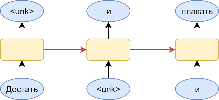
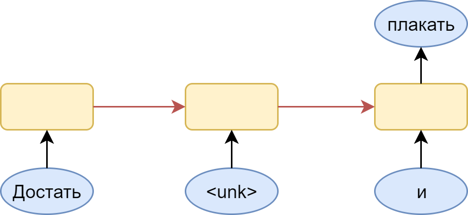
Here is a many-to-many version with a dictionary in which there is no place for the word “ink”. A logical step is the substitution for it of a special token <unk> - an unfamiliar word. The problem is that the model happily learns that after any word there may be an unfamiliar word. As a result, the distribution produced by it turns out to be shifted in the direction of this particular unfamiliar word. Of course, this is easily solved: you just need to sample from the distribution without this token, but still there is a feeling that the resulting model is somewhat crooked.
An alternative option is to use many-to-one architecture:
At the same time, it is necessary to cut all sorts of chains of words from the training set - which will lead to its noticeable swelling. But all the chains for which the following words - is unknown, we can simply pass completely solving the problem with a frequent prediction <unk> token.
This model had the following parameters (in terms of the keras library):
As you can see, it is included in the 60,000 + 1 word plus the first token is the same <unk>.
The easiest way is to repeat it with a small modification of the example . Its main difference is that the example demonstrates character-by-character text generation, while the above-described variant is based on word-by-word generation.
The resulting model really generates something, but even the grammatical consistency of the resulting sentences is often not impressive (about the semantic load and say nothing). The logical next step is to use pre-trained embeddingings for words. Their addition simplifies the learning of the model, and the connections between words learned on a large body can give meaning to the generated text.
The main problem: for Russian (as opposed to, for example, English), it is difficult to find good word form words. With the available result, it became even worse.
Let's try pochamanit a little with the model. The lack of a network, apparently - in too many parameters. The network simply does not learn. To fix this, you should work with the input and output layers - the heaviest elements of the model.
Obviously, it makes sense to reduce the dimension of the input layer. This can be achieved simply by reducing the dimension of word-form emebingov - but it is more interesting to go the other way.
Instead of representing the word in one index in a high-dimensional space, add morphological markup:
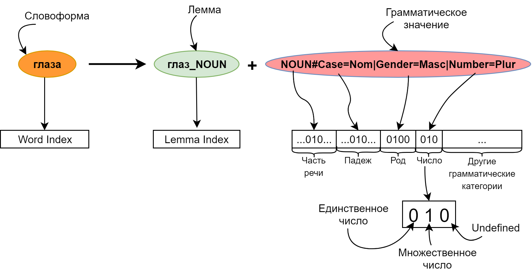
Each word will be described by a pair: its lemma and grammatical meaning. Using lemmas instead of word forms allows you to greatly reduce the size of embeddings: the first thirty thousand lemmas correspond to several hundred thousand different words. Thus, seriously reducing the input layer, we also increased the vocabulary of our model.
As can be seen from the figure, the lemma has a part of speech assigned to it. This is done in order to be able to use already pre-trained embeddings for lemmas (for example, from RusVectores ). On the other hand, embeddings for thirty thousand lemmas can be fully trained from scratch, initializing them by chance.
We presented the grammatical meaning in the format of Universal Dependencies , since I had a model at hand that was trained for Dialogue 2017 .
When applying a grammatical meaning to the input of a model, it is translated into a bit mask: for each grammatical category, positions are allocated by the number of grammes in this category - plus one position for the absence of this category in the grammatical meaning (Undefined). Bit vectors for all categories are glued together into one big vector.
Generally speaking, the grammatical meaning could, like the lemma, be represented by an index and teach embedding for it. But the bitmask network showed higher quality.
This bit vector can, of course, be submitted directly to LSTM, but it is better to pass it through one or two fully connected layers to reduce the dimension and, at the same time, to detect connections between gram patterns.
Instead of the word index, one can predict the same lemma and grammatical meaning separately. After that, you can sample the lemma from the resulting distribution and put it in a form with the most likely grammatical meaning. A small minus of such an approach is that it is impossible to guarantee the presence of such a grammatical meaning in this lemma.
This problem is easily fixed in two ways. The honest way is to sample exactly the word from the pairs of realizable lemma + grammatical meaning (the probability of this word, of course, is the product of the probabilities of the lemma and the grammatical meaning). A faster alternative is to choose the most likely grammatical meaning among the possible ones for the sampled lemma.
In addition, the softmax-layer could be replaced with a hierarchical softmax or, in general, dragged down the implementation of noise contrastive estimation from tensorflow . But we, with our dictionary size, turned out to be enough and ordinary softmax. At least, the above-mentioned tricks did not bring a significant increase in the quality of the model.
As a result, we have the following model:
So far, we have not discussed in any way the important question of what we are learning. For training, we took a large piece of stihi.ru and added morphological markup to it. After that, long lines were selected (at least five words) and trained on them.
Each line was considered as independent - thus we struggled with the fact that neighboring lines are often weakly connected in meaning (especially on stihi.ru ). Of course, you can learn at once on a complete poem, and this could give an improvement in the quality of the model. But we decided that we are faced with the task of building a network that is able to write grammatically connected text, and for such a purpose it is enough to learn only on strings.
When learning, the terminating character was added to all lines, and the order of words in the lines was inverted. Expand sentences needed to simplify the rhyming of words when generating. The final character is needed in order to start generating the sentence from it.
Among other things, for simplicity, we threw all the punctuation marks from the texts. This was done because the network noticeably retrained under commas and other ellipsis: in the sample they were put literally after each word. Of course, this is a strong omission of our model and there is hope to fix it in the next version.
Schematically, the pre-processing of texts can be depicted as follows:
The arrows indicate the direction in which the model reads the sentence.
Let us turn, finally, to the poetry generator. We began with the fact that the language model is needed only to build hypotheses about the next word. For the generator, rules are needed according to which poems will be built from a sequence of words. Such rules work as language model filters: of all the possible variants of the next word, only those that are suitable remain - in our case, by meter and rhyme.
Metric rules determine the sequence of stressed and unstressed syllables in a string. They are usually recorded in the form of a template of pros and cons: plus means a stressed syllable, and a minus corresponds to unstressed. For example, consider the metric pattern + - + - + - + - (in which one can suspect a four-stop trochee):
Generation, as already mentioned, goes from right to left - in the direction of the arrows in the picture. Thus, after mist, filters will ban the generation of such words as a blizzard (stress is not there) or bad weather (an extra syllable). If the word has more than 2 syllables, it passes the filter only when the stressed syllable does not fall on the “minus” in the metric pattern.
The second type of rules - restrictions on rhyme. It is for them that we generate poems backwards. The filter is used when generating the very first word in the line (which will be the last after the reversal). If a string has already been generated, with which the given one should rhyme, this filter will immediately cut off all non-rhymed words.
Also, an additional rule was applied prohibiting to consider rhymes of a word form with the same lemma.
You might have a question: where did we get the stress from the words, and how did we determine which words rhyme with which ones? To work with stresses, we took a large dictionary and trained a classifier on this dictionary to predict the stresses of unfamiliar words (a story that deserves a separate article). Rhyming is determined by simple heuristics based on the location of the stressed syllable and its letter composition.
As a result of the operation of the filters, there could be no words left. To solve this problem, we do a beam search (beam search), choosing at each step instead of one at once N paths with the highest probabilities.
Total, generator input parameters - language model, metric pattern, rhyme pattern, N in radial search, rhyming heuristics parameters. At the exit we have a ready poem. As a language model in the same generator, you can use the N-gram model. The filter system is easily customized and complemented.
So confusing to me now sad
What will it live
Not destined to circle on the way
Feeling the bomzhik pain
Lost somewhere in the alley
Where are you my recollections
I love you my relatives
How many lies of betrayal and flattery
Nothing else is needed
For the sins of your voice
Miss your window
And gentle esters
Love you with my warmth
You shorthand
The post was written jointly with Ilya Gusev. Elena Ivashkovskaya, Nadezhda Karatsapova and Polina Matavina also took part in the project.
The work on the generator was carried out within the framework of the course “Intellectual Systems” of the Computational Linguistics Department of the FIVT MIPT. I would like to thank the author of the course, Konstantin Anisimovich, for the advice he gave in the process.
Many thanks atwice for help in reading the article.
I love you my bride
White frost on your eyelashes
Kiss on the body wordless
Once at school, it seemed to me that writing poetry was simple: you just need to arrange the words in the right order and select the right rhyme. Traces of these hallucinations (or illusions, I do not distinguish them) met you in the epigraph. Only this poem is, of course, not the result of my then creative work, but a product of a neural network trained on the same principle.
Rather, the neural network is needed only for the first stage - the arrangement of words in the correct order. The rules applied on top of the neural network predictions cope with rhyming. Want to know more about how we implemented it? Then welcome under cat.
Language models
Definition
Let's start with the language model. On Habré, I have met not too many articles about them - it would not be superfluous to recall what kind of beast it is.
')
Language models determine the likelihood of a sequence of words
in this language: . Let us move from this terrible probability to the product of conditional probabilities of a word from an already read context: .In life, these conditional probabilities show what word we expect to see next. Let us see, for example, the well-known words from Pushkin:
The language model that sits with us (in any case, with me) in my head suggests: after honest ones mine is unlikely to go again. And here, and, of course, the rules - very much so.
N-gram language models
It seems the easiest way to build such a model is to use N-gram statistics. In this case, we approximate the probability
- rejecting words that are too far away as they do not affect the probability of a given occurrence.Such a model is easily implemented with the help of Counter on Python - and it turns out to be very heavy and not too variable. One of its most noticeable problems is the lack of statistics: most of the 5-gram words, including those permissible by the language, simply cannot be found in any large body.
To solve such a problem, Kneser – Ney or Katz's backing-off is usually used. For more information on N-gram smoothing methods, refer to Christopher Manning's famous book “Foundations of Statistical Natural Language Processing”.
I want to note that I called the 5-grams of words for a reason: it is them (with anti-aliasing, of course) that Google demonstrates in the article “One Billion Word Benchmark for Measuring Progress in Statistical Language Modeling” - and it shows results that are quite comparable to those of recurrent neural networks - which, in fact, will be discussed further.
Neural Network Language Models
The advantage of recurrent neural networks is the ability to use an infinitely long context. Together with each word arriving at the input of a recurrent cell, a vector appears in it representing the entire previous history — all the words processed to a given moment (the red arrow in the picture).
The possibility of using the context of unlimited length is, of course, only conditional. In practice, classic RNNs suffer from gradient damping - in fact, the inability to remember the context further than a few words. To combat this, special memory cells were invented. The most popular are LSTM and GRU. In the following, speaking of the recurrent layer, I will always mean LSTM.
The red arrow in the picture shows the display of the word in its embedding. The output layer (in the simplest case) is a fully connected layer with a size corresponding to the size of the dictionary, having softmax activation — to obtain a probability distribution for the vocabulary words. From this distribution, you can sample the next word (or just take the maximum possible).
Already in the picture you can see a minus of such a layer: its size. With a dictionary of several hundred thousand words, he can easily stop getting on a video card, and his body requires huge corpus of texts. This is very clearly demonstrates the picture from the blog torch :
To combat this, a very large number of different techniques were invented. The most popular are hierarchical softmax and noise contrastive estimation. Details about these and other methods should be read in the excellent article Sebastian Ruder .
Language Model Assessment
A more or less standard loss function, optimized for multi-class classification, is the cross-entropy loss function. In general, cross-entropy between vectors
and the predicted vector recorded as . It shows the proximity of the distributions given by and .When calculating cross-entropy for multi-class classification
- this is the probability first class, and - a vector obtained with one-hot-encoding (i.e., a bit vector in which a single unit is at the position corresponding to the class number). Then with some .Cross-entropy loss of the whole sentence
are obtained by averaging the values over all words. They can be written as: . It can be seen that this expression corresponds to what we want to achieve: the probability of a real sentence from the language should be as high as possible.In addition, perplexity is a metric specific to language modeling:
.To understand its meaning, let's look at a model that predicts words from the dictionary equally likely, regardless of context. For her
where N is the size of the dictionary, and the perplexion will be equal to the size of the dictionary - N. Of course, this is a completely stupid model, but looking back at it, you can interpret the perplexion of real models as the level of ambiguity of word generation.For example, in the model with perplexia 100, the choice of the next word is also ambiguous, as the choice of a uniform distribution among 100 words. And if such perplexion was achieved on a dictionary of 100,000, it turns out that we managed to reduce this ambiguity by three orders of magnitude compared to the “stupid” model.
The implementation of the language model for the generation of poems
Building a network architecture
Recall now that for our task a language model is needed to select the most appropriate next word by the already generated sequence. And from this it follows that in predicting you will never meet unfamiliar words (well, where will they come from). Therefore, the number of words in the dictionary remains entirely in our power, which allows you to adjust the size of the resulting model. Thus, we had to forget about such human achievements as symbolic embeddings for representing words (you can read about them, for example, here ).
Based on these prerequisites, we started with a relatively simple model, generally repeating the one shown in the picture above. Two yellow LSTM layers followed by a fully connected layer acted as a yellow rectangle.
The decision to limit the size of the output layer seems quite working. Naturally, the dictionary should be limited in frequency - say, taking fifty thousand of the most frequent words. But here another question arises: which architecture of the recurrent network is better to choose.
There are two obvious options: use the many-to-many option (for each word, try to predict the following) or many-to-one (predict the word by the sequence of the preceding words).
To better understand the essence of the problem, look at the picture:
Here is a many-to-many version with a dictionary in which there is no place for the word “ink”. A logical step is the substitution for it of a special token <unk> - an unfamiliar word. The problem is that the model happily learns that after any word there may be an unfamiliar word. As a result, the distribution produced by it turns out to be shifted in the direction of this particular unfamiliar word. Of course, this is easily solved: you just need to sample from the distribution without this token, but still there is a feeling that the resulting model is somewhat crooked.
An alternative option is to use many-to-one architecture:
At the same time, it is necessary to cut all sorts of chains of words from the training set - which will lead to its noticeable swelling. But all the chains for which the following words - is unknown, we can simply pass completely solving the problem with a frequent prediction <unk> token.
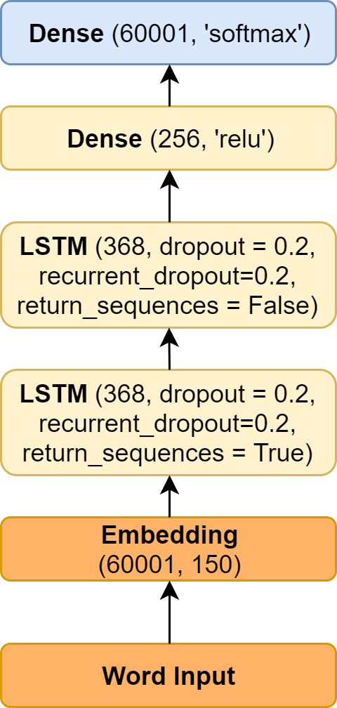
This model had the following parameters (in terms of the keras library):
As you can see, it is included in the 60,000 + 1 word plus the first token is the same <unk>.
The easiest way is to repeat it with a small modification of the example . Its main difference is that the example demonstrates character-by-character text generation, while the above-described variant is based on word-by-word generation.
The resulting model really generates something, but even the grammatical consistency of the resulting sentences is often not impressive (about the semantic load and say nothing). The logical next step is to use pre-trained embeddingings for words. Their addition simplifies the learning of the model, and the connections between words learned on a large body can give meaning to the generated text.
The main problem: for Russian (as opposed to, for example, English), it is difficult to find good word form words. With the available result, it became even worse.
Let's try pochamanit a little with the model. The lack of a network, apparently - in too many parameters. The network simply does not learn. To fix this, you should work with the input and output layers - the heaviest elements of the model.
Completion of the input layer
Obviously, it makes sense to reduce the dimension of the input layer. This can be achieved simply by reducing the dimension of word-form emebingov - but it is more interesting to go the other way.
Instead of representing the word in one index in a high-dimensional space, add morphological markup:
Each word will be described by a pair: its lemma and grammatical meaning. Using lemmas instead of word forms allows you to greatly reduce the size of embeddings: the first thirty thousand lemmas correspond to several hundred thousand different words. Thus, seriously reducing the input layer, we also increased the vocabulary of our model.
As can be seen from the figure, the lemma has a part of speech assigned to it. This is done in order to be able to use already pre-trained embeddings for lemmas (for example, from RusVectores ). On the other hand, embeddings for thirty thousand lemmas can be fully trained from scratch, initializing them by chance.
We presented the grammatical meaning in the format of Universal Dependencies , since I had a model at hand that was trained for Dialogue 2017 .
When applying a grammatical meaning to the input of a model, it is translated into a bit mask: for each grammatical category, positions are allocated by the number of grammes in this category - plus one position for the absence of this category in the grammatical meaning (Undefined). Bit vectors for all categories are glued together into one big vector.
Generally speaking, the grammatical meaning could, like the lemma, be represented by an index and teach embedding for it. But the bitmask network showed higher quality.
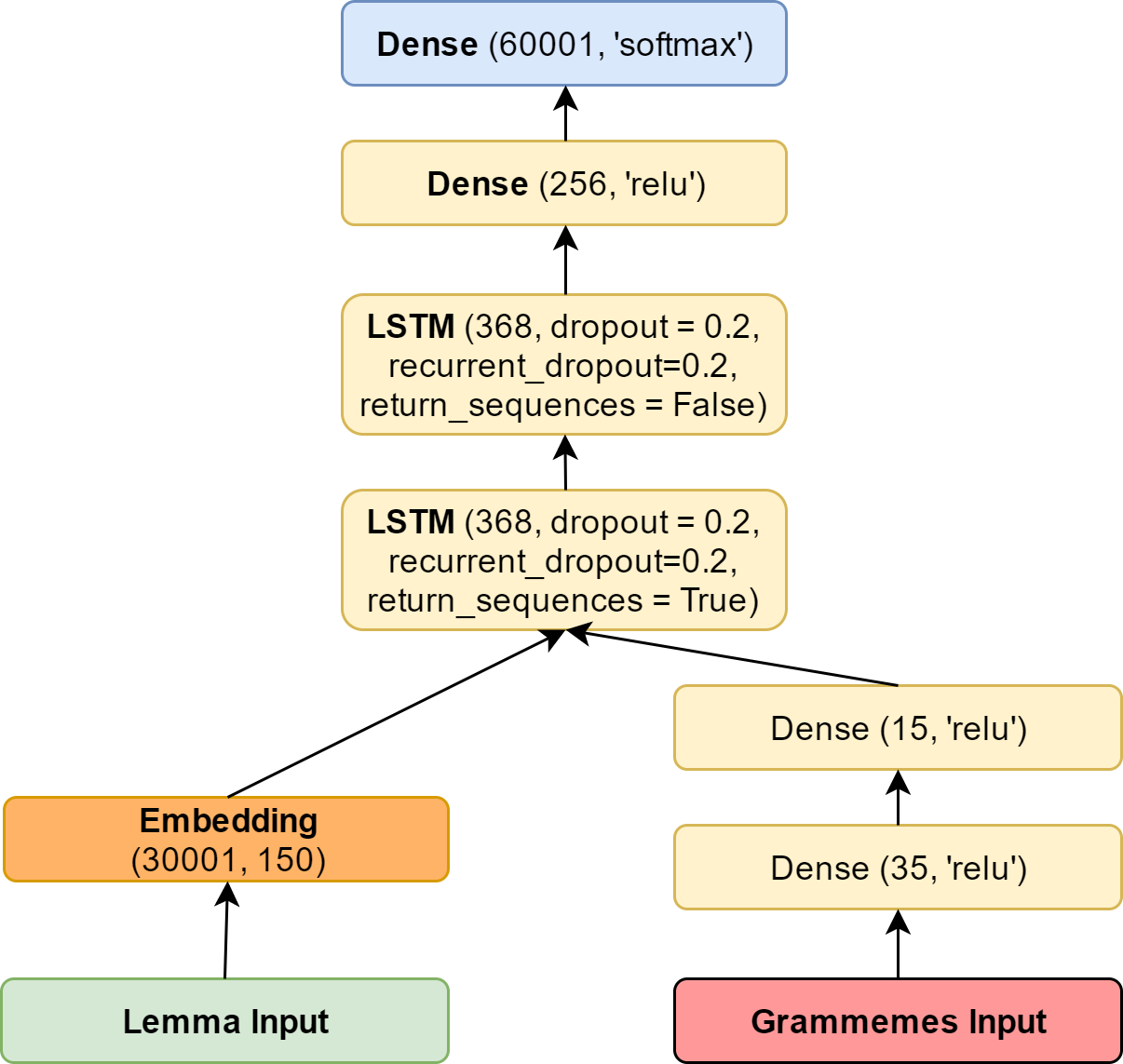
This bit vector can, of course, be submitted directly to LSTM, but it is better to pass it through one or two fully connected layers to reduce the dimension and, at the same time, to detect connections between gram patterns.
Finalization of the output layer
Instead of the word index, one can predict the same lemma and grammatical meaning separately. After that, you can sample the lemma from the resulting distribution and put it in a form with the most likely grammatical meaning. A small minus of such an approach is that it is impossible to guarantee the presence of such a grammatical meaning in this lemma.
This problem is easily fixed in two ways. The honest way is to sample exactly the word from the pairs of realizable lemma + grammatical meaning (the probability of this word, of course, is the product of the probabilities of the lemma and the grammatical meaning). A faster alternative is to choose the most likely grammatical meaning among the possible ones for the sampled lemma.
In addition, the softmax-layer could be replaced with a hierarchical softmax or, in general, dragged down the implementation of noise contrastive estimation from tensorflow . But we, with our dictionary size, turned out to be enough and ordinary softmax. At least, the above-mentioned tricks did not bring a significant increase in the quality of the model.
Final model
As a result, we have the following model:
Training data
So far, we have not discussed in any way the important question of what we are learning. For training, we took a large piece of stihi.ru and added morphological markup to it. After that, long lines were selected (at least five words) and trained on them.
Each line was considered as independent - thus we struggled with the fact that neighboring lines are often weakly connected in meaning (especially on stihi.ru ). Of course, you can learn at once on a complete poem, and this could give an improvement in the quality of the model. But we decided that we are faced with the task of building a network that is able to write grammatically connected text, and for such a purpose it is enough to learn only on strings.
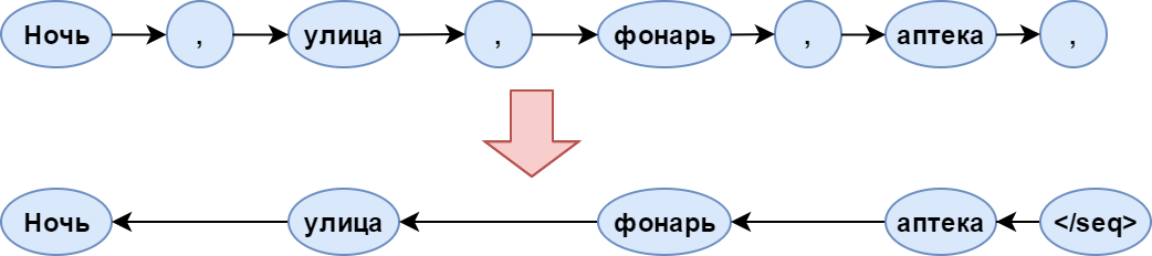
When learning, the terminating character was added to all lines, and the order of words in the lines was inverted. Expand sentences needed to simplify the rhyming of words when generating. The final character is needed in order to start generating the sentence from it.
Among other things, for simplicity, we threw all the punctuation marks from the texts. This was done because the network noticeably retrained under commas and other ellipsis: in the sample they were put literally after each word. Of course, this is a strong omission of our model and there is hope to fix it in the next version.
Schematically, the pre-processing of texts can be depicted as follows:
The arrows indicate the direction in which the model reads the sentence.
Generator implementation
Filter Rules
Let us turn, finally, to the poetry generator. We began with the fact that the language model is needed only to build hypotheses about the next word. For the generator, rules are needed according to which poems will be built from a sequence of words. Such rules work as language model filters: of all the possible variants of the next word, only those that are suitable remain - in our case, by meter and rhyme.
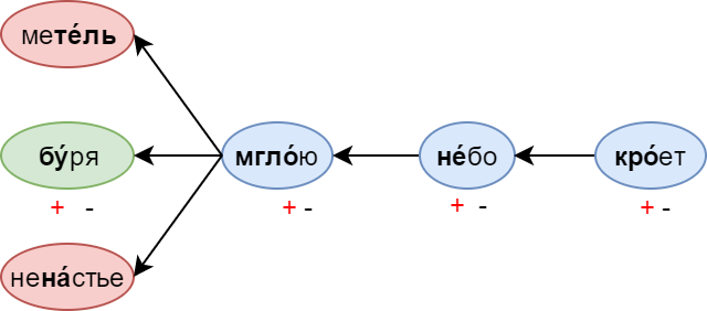
Metric rules determine the sequence of stressed and unstressed syllables in a string. They are usually recorded in the form of a template of pros and cons: plus means a stressed syllable, and a minus corresponds to unstressed. For example, consider the metric pattern + - + - + - + - (in which one can suspect a four-stop trochee):
Generation, as already mentioned, goes from right to left - in the direction of the arrows in the picture. Thus, after mist, filters will ban the generation of such words as a blizzard (stress is not there) or bad weather (an extra syllable). If the word has more than 2 syllables, it passes the filter only when the stressed syllable does not fall on the “minus” in the metric pattern.
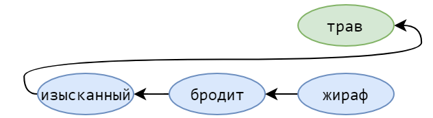
The second type of rules - restrictions on rhyme. It is for them that we generate poems backwards. The filter is used when generating the very first word in the line (which will be the last after the reversal). If a string has already been generated, with which the given one should rhyme, this filter will immediately cut off all non-rhymed words.
Also, an additional rule was applied prohibiting to consider rhymes of a word form with the same lemma.
You might have a question: where did we get the stress from the words, and how did we determine which words rhyme with which ones? To work with stresses, we took a large dictionary and trained a classifier on this dictionary to predict the stresses of unfamiliar words (a story that deserves a separate article). Rhyming is determined by simple heuristics based on the location of the stressed syllable and its letter composition.
Beam search
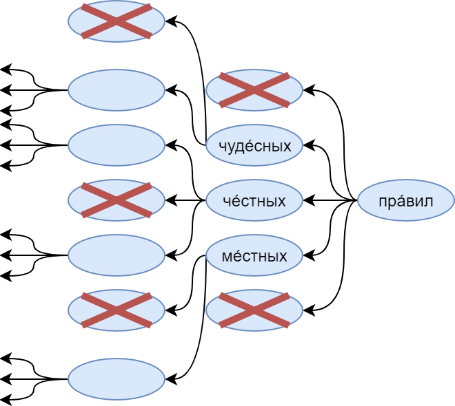
As a result of the operation of the filters, there could be no words left. To solve this problem, we do a beam search (beam search), choosing at each step instead of one at once N paths with the highest probabilities.
Total, generator input parameters - language model, metric pattern, rhyme pattern, N in radial search, rhyming heuristics parameters. At the exit we have a ready poem. As a language model in the same generator, you can use the N-gram model. The filter system is easily customized and complemented.
Examples of poems
So confusing to me now sad
What will it live
Not destined to circle on the way
Feeling the bomzhik pain
Lost somewhere in the alley
Where are you my recollections
I love you my relatives
How many lies of betrayal and flattery
Nothing else is needed
For the sins of your voice
Miss your window
And gentle esters
Love you with my warmth
You shorthand
Links
- Repository
- Package in pypi
- Public in VK with verses
- Model and dictionaries necessary for her work
- Oxford NLP course prepared with the participation of DeepMind
- One Billion Word Benchmark for Measuring Progress in Statistical Language Modeling
- Exploring the Limits of Language Modeling
- Character-Aware Neural Language Models
The post was written jointly with Ilya Gusev. Elena Ivashkovskaya, Nadezhda Karatsapova and Polina Matavina also took part in the project.
The work on the generator was carried out within the framework of the course “Intellectual Systems” of the Computational Linguistics Department of the FIVT MIPT. I would like to thank the author of the course, Konstantin Anisimovich, for the advice he gave in the process.
Many thanks atwice for help in reading the article.
Source: https://habr.com/ru/post/334046/
All Articles