Creating a GLSL smoke shader

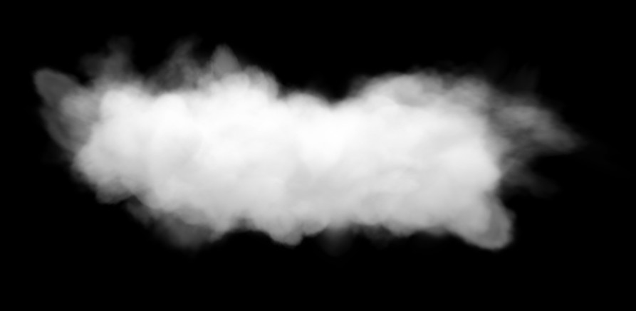
[The smoke on the KDPV is somewhat more complicated than that obtained in the tutorial.]

Smoke has always been surrounded by a halo of mystery. It's nice to look at him, but it's hard to model. Like many other physical phenomena, smoke is a chaotic system that is very difficult to predict. The simulation state is highly dependent on the interaction between the individual particles.

That is why it is so difficult to process it in a video processor: the smoke can be divided into the behavior of a single particle, repeated millions of times in different places.
')
In this tutorial, I will talk in detail about creating a smoke shader from scratch and teach you some useful shader design techniques so that you can expand your arsenal and create your own effects.

What we learn

Here is the final result we will strive for:


We implement the algorithm described in the work of Jos Stam on the dynamics of liquids in games in real time . In addition, we learn how to render into texture , this technique is also called frame buffers . It is very useful in programming shaders, because it allows you to create many effects.

Training

The examples and code implementations of this tutorial use JavaScript and ThreeJS , but you can use it on any platform with shader support. (If you are unfamiliar with the basics of programming, then you should study this tutorial .)

All code samples are stored on CodePen, but they can also be found in the GitHub repository linked to the article (there it may be easier to read the code).

Theory and Foundations

The algorithm from the work of Jos Stam gives priority to speed and visual quality to the detriment of physical accuracy, this is what we need in games.

This job may seem much more difficult than it actually is, especially if you are not familiar with differential equations. However, the meaning of the technique is summarized in this figure:


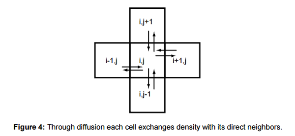
Thanks to scattering, each cell exchanges its density with its neighbors.

This is all that is needed to create a realistic looking smoke effect: the value in each cell at each iteration “dissipates” into all its neighboring cells. This principle is not always clear immediately, if you want to experiment with an example, you can explore the interactive demo :


View an interactive demo on CodePen .

When you click on any cell, it is assigned the value 100 . You see how each cell gradually transfers its value to its neighbors. The easiest way to see this is by clicking Next to view individual frames. Toggle Display Mode to see how it will look when these numbers correspond to color values.

The above demo runs on the central processor, the loop goes through each cell. Here’s what this cycle looks like:

 //W =     //H =   //f =  / //     newGrid,    ,       for(var r=1; r<W-1; r++){ for(var c=1; c<H-1; c++){ newGrid[r][c] += f * ( gridData[r-1][c] + gridData[r+1][c] + gridData[r][c-1] + gridData[r][c+1] - 4 * gridData[r][c] ); } } 

This code snippet is the basis of the algorithm. Each cell receives a part of the values ​​of the four neighboring cells minus its own value, where f is a coefficient less than 1. We multiply the current value of the cell by 4 so that it dissipates from high to low values.

To make this clear, consider the following situation:



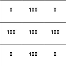
Take a cell in the middle (at position [1,1] in the grid) and apply the above scattering equation. Suppose that f is 0.1 :

 0.1 * (100+100+100+100-4*100) = 0.1 * (400-400) = 0 

No scattering occurs because all cells have the same values!

Then consider the cell in the upper left corner (we assume that the values ​​of all the cells outside the grid shown are 0 ):

 0.1 * (100+100+0+0-4*0) = 0.1 * (200) = 20 

So, now we have a net gain of 20! Let's look at the last case. After one time step (after applying this formula to all cells), our grid will look like this:



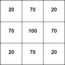
Let's look again at the scatter in the middle cell :

 0.1 * (70+70+70+70-4*100) = 0.1 * (280 - 400) = -12 

We got a net decrease of 12! Therefore, the values ​​always change from large to small.

Now, if we want more realism, we need to reduce the size of the cells (which can be done in the demo), but at a certain stage everything will start to slow down a lot, because we have to consistently pass through each cell. Our goal is to write this algorithm in a shader that can use the power of a video processor to process all cells (like pixels) simultaneously and in parallel.

So, to summarize: our common technique is that each pixel, each frame loses some of its color value and passes it to neighboring pixels. Sounds easy, right? Let's implement this system and see what happens!

Implementation

We start with a basic shader that draws the entire screen. To make sure that it works, we will try to paint over the screen with a solid black color (or any other). Here’s what the scheme I use in Javascript looks like.


Click the buttons at the top to see the HTML, CSS and JS code.

Our shader is simple:

 uniform vec2 res; void main() { vec2 pixel = gl_FragCoord.xy / res.xy; gl_FragColor = vec4(0.0,0.0,0.0,1.0); } 

res and pixel tell us the coordinates of the current pixel. We pass the screen sizes to res as a uniform variable. (While we do not use them, but soon they will be useful.)

Step 1: Move Values ​​Between Pixels

I repeat once again what we want to implement:

Our common technique is that each pixel each frame loses a part of its color value and transmits it to neighboring pixels.

In this formulation, the implementation of the shader is impossible . Do you understand why? Remember, the only thing that a shader can do is return the color value of the current pixel being processed. That is, we need to reformulate the task in such a way that the solution affects only the current pixel. We can say:

Each pixel should get a little color of its neighbors and lose a little of its own.

Now this solution can be implemented. However, if you try to do this, then we will come across a fundamental problem ...

Consider a simpler case. Suppose we need a shader, gradually repainting the image in red. You can write the following shader:

 uniform vec2 res; uniform sampler2D texture; void main() { vec2 pixel = gl_FragCoord.xy / res.xy; gl_FragColor = texture2D( tex, pixel );//     gl_FragColor.r += 0.01;//    } 

It can be expected that each frame of the red component of each pixel will increase by 0.01 . Instead, we get a static image, in which all the pixels are just a little redder than at the beginning. The red component of each pixel will increase only once, despite the fact that the shader is executed every frame.

Do you understand why this happens?

Problem

The problem is that any operation that we perform with a shader is transmitted to the screen, and then disappears forever. Now our process looks like this:



We pass in uniform variables and texture to the shader, it makes the pixels a little redder, draws them on the screen, and then it starts all over again. Everything we draw in the shader is cleared by the next draw step.

We need something like this:



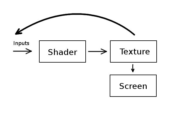
Instead of direct rendering onto the screen, we can draw pixels into the texture, and then draw that texture on the screen. The screen will display the same image, except that we can now send the output as input. So you can get shaders that accumulate or distribute values, rather than just dropping each frame. This is what is called “frame buffer focus.”

Focus with frame buffer

Common technology will be the same for all platforms. Go “render to texture” for any language or tool you are using and learn the implementation details. You can also see how to use frame buffer objects , which are just another name for rendering to a buffer instead of a screen.

In ThreeJS, the analogue of this function is WebGLRenderTarget . That is what we will use as an intermediate texture for rendering. However, there is a small obstacle: you can not read and render in one texture at the same time . The easiest way around this limitation is to use two textures.

Let A and B be the two textures we created. Then the method will be as follows:

1. We transfer A through a shader, we render in B.
2. Render B to the screen.
3. Pass B through the shader, render it in A.
4. Render A to the screen.
5. Repeat 1.

A shorter code will be as follows:

1. We transfer A through a shader, we render in B.
2. Render B to the screen.
3. Change A and B (that is, variable A now contains the texture found in B, and vice versa).
4. Repeat 1.

That's all. Here is the implementation of this algorithm in ThreeJS:


The new shader code is in the HTML tab.

We still see the black screen from which we started. The shader is also not too different:

 uniform vec2 res; //     uniform sampler2D bufferTexture; //   void main() { vec2 pixel = gl_FragCoord.xy / res.xy; gl_FragColor = texture2D( bufferTexture, pixel ); } 

In addition, now we have added this line ( test! ):

 gl_FragColor.r += 0.01; 

You will see that the screen gradually turns red. This is a rather important step, so we can briefly dwell on it and compare it with how the algorithm worked initially.

Task: What happens if we gl_FragColor.r += pixel.x; in the frame buffer example, unlike the original example? Think a little about why the results are different, and why they are just like that.

Step 2: get the smoke source

Before we make everything move, we need to find a way to create smoke. The simplest way is to manually fill in an arbitrary area in the shader with white.

 //         float dist = distance(gl_FragCoord.xy, res.xy/2.0); if(dist < 15.0){ //    15  gl_FragColor.rgb = vec3(1.0); } 

If we want to check the correctness of the frame buffer, we can try to add to the color value, and not just assign it. You will see that the circle is gradually becoming whiter.

 //         float dist = distance(gl_FragCoord.xy, res.xy/2.0); if(dist < 15.0){ //    15  gl_FragColor.rgb += 0.01; } 

Another way is to replace this fixed point with the position of the mouse. We can pass the third value indicating whether the mouse button is down. This way we can create smoke by pressing the left key. Here is the implementation of this feature:


Click to create smoke.

This is what our shader looks like:

 //     uniform vec2 res; //   uniform sampler2D bufferTexture; // x,y -  . z -  / uniform vec3 smokeSource; void main() { vec2 pixel = gl_FragCoord.xy / res.xy; gl_FragColor = texture2D( bufferTexture, pixel ); //         float dist = distance(smokeSource.xy,gl_FragCoord.xy); //  ,     if(smokeSource.z > 0.0 && dist < 15.0){ gl_FragColor.rgb += smokeSource.z; } } 

Task: do not forget that branching (conditional transitions) are usually expensive in shaders. Can you rewrite the shader without using the if construct? (The solution is in CodePen.)

If you do not understand, then in the previous tutorial there is a detailed explanation of using the mouse in shaders (in the part about lighting).

Step 3: Dissipate Smoke

Now the simple, but the most interesting part! We put everything together, we finally had to tell the shader: each pixel should receive some of the color from its neighbors, and lose some of its own.

It expresses something like this:

 //   float xPixel = 1.0/res.x; //    float yPixel = 1.0/res.y; vec4 rightColor = texture2D(bufferTexture,vec2(pixel.x+xPixel,pixel.y)); vec4 leftColor = texture2D(bufferTexture,vec2(pixel.x-xPixel,pixel.y)); vec4 upColor = texture2D(bufferTexture,vec2(pixel.x,pixel.y+yPixel)); vec4 downColor = texture2D(bufferTexture,vec2(pixel.x,pixel.y-yPixel)); //   gl_FragColor.rgb += 14.0 * 0.016 * ( leftColor.rgb + rightColor.rgb + downColor.rgb + upColor.rgb - 4.0 * gl_FragColor.rgb ); 

The f coefficient remains the same. In this case, we have a time step ( 0.016 , that is, 1/60, because the program runs at 60 fps), and I picked up different numbers until I stopped at a value of 14 , which looks good. Here is the result:

Oh, oh, it's all stuck!

This is the same scattering equation that we used in the demo for the CPU, but our simulation stops! What is the reason?

It turns out that textures (like all numbers in a computer) have limited accuracy. At some point, the coefficient we subtract becomes too small and rounds to 0, so the simulation stops. To fix this, we need to check that it does not fall below any minimum value:

 float factor = 14.0 * 0.016 * (leftColor.r + rightColor.r + downColor.r + upColor.r - 4.0 * gl_FragColor.r); //       float minimum = 0.003; if (factor >= -minimum && factor < 0.0) factor = -minimum; gl_FragColor.rgb += factor; 

I use the component r instead of rgb to get the coefficient, because it is easier to work with individual numbers and because all the components still have the same values ​​(because the smoke is white).

Through trial and error, I found that a good threshold is 0.003 , at which the program does not stop. My only concern is the coefficient with a negative value in order to guarantee its constant decrease. By adding this fix, we get the following:

Step 4: Smoke Up

But it still doesn’t look like smoke. If we want it to go up, and not in all directions, we need to add weights. If the lower pixels always influence more than other directions, then the pixels will seem to rise up.

Experimenting with the coefficients, we can choose what looks very decent in this equation:

 //   float factor = 8.0 * 0.016 * ( leftColor.r + rightColor.r + downColor.r * 3.0 + upColor.r - 6.0 * gl_FragColor.r ); 

And this is what a shader looks like:

Note on the scattering equation

I just played with the coefficients so that the rising smoke looked beautiful. You can make him move in any other direction.

It is important to add that it is very simple to “blow up” the simulation. (Try changing the value of 6.0 to 5.0 and see what happens.) Obviously, this is due to the fact that cells gain more than they lose.

This equation is actually referred to in my work as the “poor dispersion” model. There is another equation in the work that is more stable, but it is not very convenient for us, mainly because it needs to write to the grid from which we read. In other words, we need to read and write one texture at a time.

What we have is enough for our purposes, but if you are interested, you can study the explanation in the paper. In addition, another equation is implemented in an interactive demo for the CPU , see the diffuse_advanced() function.

Minor fix

You may have noticed that when creating smoke at the bottom of the screen, it gets stuck there. This is because the pixels on the bottom line try to get values ​​from the nonexistent pixels below them.

To fix this, we will let the bottom pixels find 0 below them:

 //    //        if(pixel.y <= yPixel){ downColor.rgb = vec3(0.0); } 

In the demo for the CPU, I coped with this by simply making sure that the lower cells do not dissipate. You can also manually set all cells beyond 0 . (The grid in the demo for the CPU goes out in one direction and one column in all directions, that is, we never see the boundaries)

Speed ​​grid

Congratulations! Now you have a ready smoke shader! In the end, I would like to briefly describe the velocity field mentioned in the paper.


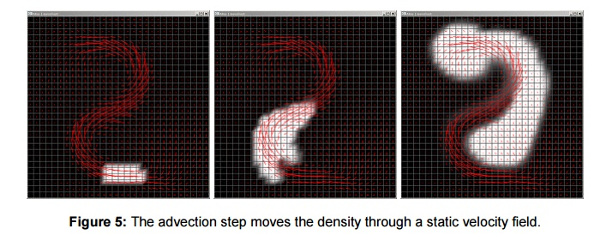
The transfer (advection) stage moves the density along a static velocity field.

Smoke is not obliged to dissipate equally upwards or in any other direction, it may follow a general pattern, for example, the one shown in the figure. You can implement this by sending another texture in which the color values ​​represent the direction in which the smoke should move at the current point. This is similar to using a normal map to indicate the direction of each pixel in the lighting tutorial.

In fact, the speed texture also does not have to be static! You can use frame buffer focus to change speeds in real time. I will not talk about this in the tutorial, but this feature has great potential for research.

Conclusion

The most important thing to learn from this tutorial: the ability to render into texture instead of a screen is a very useful technique.

What can frame buffers be useful for?

They are often used for post-processing in games. If you want to apply a color filter, instead of using it with each object, you can render all the objects into a texture to fit the screen, and then apply a shader to this texture and draw it on the screen.

Another use case is the implementation of shaders that require multiple passes. for example blur . Usually, the image is passed through a shader, blurred along the x axis, and then passed through again to blur the y axis.

The last example is deferred rendering , which we discussed in the previous tutorial . This is an easy way to efficiently add multiple light sources to the scene. The great thing about this is that the calculation of lighting no longer depends on the number of light sources.

Do not be afraid of technical articles.

Much more details can be found in the work I have cited. It requires familiarity with linear algebra, but let it not hurt you to analyze and try to implement the system. The essence of it is quite simple to implement (after some adjustment of the coefficients).

I hope that you learned a little more about shaders and the article turned out to be useful.