K-sort: a new algorithm that exceeds the pyramid when n <= 7 000 000
From the translator. Translation of the 2011 article (amendment, sent on July 19, 2011) to arxiv.org on the statistical analysis of a quick sort modification. Surely there are people who use the described version intuitively. Here is the mathematical justification of efficiency with n <= 7 000 000
Keywords
')
Internal sorting; Uniform distribution; Medium temporal complexity; Statistical analysis; Statistical evaluation
Sundarajan and Chakraborty [10] presented a new version of quick sorting that removes exchanges. Crazat [1] noted that the algorithm competes well with some other versions of quick sorting. However, it uses an auxiliary array, increasing spatial complexity. Here we provide the second version where we removed the auxiliary array. This version, which we call K-sort, orders the elements faster than the pyramid with a significant array size (n <= 7 000 000) for the input data of the uniform distribution U [0, 1].
1. Introduction
There are several internal sorting methods (where all items can be stored in main memory). The simplest algorithms, such as bubble sorting, usually take O (n 2 ) time ordering n objects and are only useful for small sets. One of the most popular algorithms for large sets is Quick sort, which occupies O (n * log 2 n) on average and O (n 2 ) in the worst case. Read more about sorting algorithms in Knut [2].
Sundarajan and Chakraborty [10] presented a new version of quick sorting that removes exchanges. Crazeat [1] found that this algorithm competes well with some other versions of Quick sort, such as SedgewickFast, Bsort and Singleton sort for n [3000..200 000]. Since the comparison algorithm predominates over exchanges, deleting exchanges does not make the complexity of this algorithm different from the complexity of the classical quick sort. In other words, our algorithm has an average and worst complexity, comparable to Quick sort, that is, O (n * log 2 n) and O (n 2 ), respectively, which is also confirmed by Crazat [1]. However, it uses an auxiliary array, thereby increasing spatial complexity. Here we offer the second improved version of our sort, which we call K-sort, where the auxiliary array is removed. It was found that the sorting of elements with K-sort is faster than the pyramid when the array size is significant (n <= 7 000 000) of uniformly distributed input U [0, 1].
1.1 K-sort
Note. If the auxiliary array has one value, it does not need to be processed.
2. Empirical (average time complexity)
A computer experiment is a series of code runs for various inputs (see Saks [9]). Conducting computer experiments at Borland International Turbo 'C ++' 5.02 , we could compare the average sorting time in seconds (the average took over 500 readings) for different values of n for K-sort and Heap. Using the Monte Carlo simulation (see Kennedy and Gentle [7]), an array of size n was filled with independent continuous uniform U [0, 1] variations, and copied into another array. These arrays were sorted by comparable algorithms. Table 1 and Fig. 1 shows empirical results.
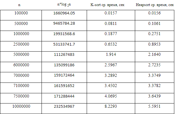
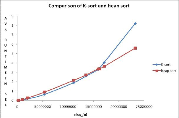
Fig. 1 Comparison Chart
The observed average times from the continuous uniform distribution of U (0,1) for the considered sorts are presented in table 1. Figure 1, together with table 1, show a comparison of the algorithms.
The points on the graph constructed from Table 1 show that the average execution time for K-sorting is less than that of the heap sort when the size of the array is less than or equal to 7,000,000 elements, and above this range Heapsort runs faster.
3. Statistical analysis of empirical results using Minitab version 15
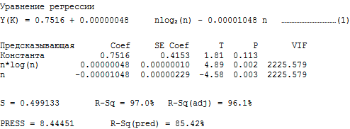
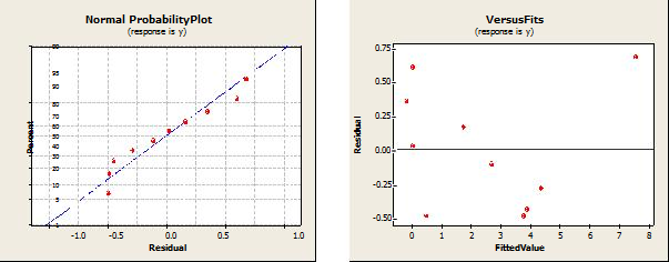
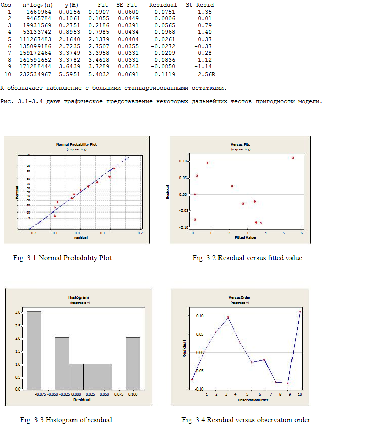
3.1. Analysis for K-sort: Regression of the average sorting time y (K) by n * log 2 (n) and n

R stands for observation with large standardized residues.
Fig. 2.1-2.4 shows a visual result of some additional model tests.

4. Discussion part
It is easy to see that the sum of squares contributed by n * log (n) to the regression model in both the K-sort sort and Heap is significant compared to the sum obtained by n. Recall that both algorithms have an average complexity of O (n * log 2 n). Thus, the experimental results confirm the theory. We saved the n-term in the model, because looking at the mathematical operator, resulting in O (nlog 2 n) complexity in the Quick sort and Heap sort, implies the n-term (see Knuth [2]).
The comparative regression equation for the average case is obtained simply by subtracting y (H) from y (K).
We have, y (K) - y (H) = 0.52586 + 0.00000035 n * log2 (n) - 0.00000792 n …… .. (3)
The advantage of equations (1), (2) and (3) is that we can predict the average execution time of both sorting algorithms, as well as their difference even for huge values of n, which are cumbersome to perform. Such a “cheap prediction” is the motto in computer experiments and allows us to carry out stochastic modeling even for non-random data. Another advantage is that you only need to know the size of the input to make a prediction. That is, the entire input (for which the answer is fixed) is not required. Thus, the prediction through the stochastic model is not only cheap, but also more efficient (Sachs, [9]).
It is important to note that when we directly work on the program execution time, we actually calculate the statistical estimate in a finite range (a computer experiment cannot be performed to enter an infinite size). Statistical evaluation differs from mathematical evaluation in the sense that, unlike mathematical evaluation, it weighs and does not accurately calculate computational operations and, as such, is able to mix different operations into conceptual evaluation, while mathematical complexity is specific to the operation. Here, the operation time is taken as its weight. For a general discussion of statistical evaluation, including formal definition and other properties, see Chakraborty and Subic [5]. See also Chakraborty, Modi and Panigraha [4] to understand why statistical evaluation is the ideal boundary for parallel computations. The assumption of statistical evaluation is obtained by running computer experiments where numerical values are assigned to weights in a finite range. This means that the credibility of the bound estimate depends on the proper development and analysis of our computer experiment. Related literature on computer experiments with other applications, such as VLSI design, burning, heat transfer, etc., can be found in (Fang, Li and Sugyanto, [3]). See also the review (Chakraborty [6]).
5. Conclusion and suggestions for future work
K-sort is obviously faster than Heap for the number of sorting elements up to 7,000,000, although both algorithms have the same order of complexity O (n * log 2 n) in the average case. Future work includes the study of parameterized complexity (Mahmoud, [8]) for this improved version. As a final comment, we highly recommend K-sort for at least n <= 7,000,000.
Nevertheless, we agree to choose Heap-sort in the worst case because it supports the complexity of O (n * log 2 n) even in the worst case, although it is more difficult to program it.
NB Continuation of work, 2012
Briefly about the main thing
Keywords
')
Internal sorting; Uniform distribution; Medium temporal complexity; Statistical analysis; Statistical evaluation
Sundarajan and Chakraborty [10] presented a new version of quick sorting that removes exchanges. Crazat [1] noted that the algorithm competes well with some other versions of quick sorting. However, it uses an auxiliary array, increasing spatial complexity. Here we provide the second version where we removed the auxiliary array. This version, which we call K-sort, orders the elements faster than the pyramid with a significant array size (n <= 7 000 000) for the input data of the uniform distribution U [0, 1].
1. Introduction
There are several internal sorting methods (where all items can be stored in main memory). The simplest algorithms, such as bubble sorting, usually take O (n 2 ) time ordering n objects and are only useful for small sets. One of the most popular algorithms for large sets is Quick sort, which occupies O (n * log 2 n) on average and O (n 2 ) in the worst case. Read more about sorting algorithms in Knut [2].
Sundarajan and Chakraborty [10] presented a new version of quick sorting that removes exchanges. Crazeat [1] found that this algorithm competes well with some other versions of Quick sort, such as SedgewickFast, Bsort and Singleton sort for n [3000..200 000]. Since the comparison algorithm predominates over exchanges, deleting exchanges does not make the complexity of this algorithm different from the complexity of the classical quick sort. In other words, our algorithm has an average and worst complexity, comparable to Quick sort, that is, O (n * log 2 n) and O (n 2 ), respectively, which is also confirmed by Crazat [1]. However, it uses an auxiliary array, thereby increasing spatial complexity. Here we offer the second improved version of our sort, which we call K-sort, where the auxiliary array is removed. It was found that the sorting of elements with K-sort is faster than the pyramid when the array size is significant (n <= 7 000 000) of uniformly distributed input U [0, 1].
1.1 K-sort
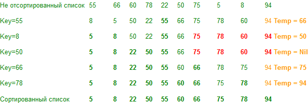
Step-1: Initialize the first element of the array as the key element and i as left, j as (right+1), k = p where p is (left+1). Step-2: Repeat step-3 till the condition (ji) >= 2 is satisfied. Step-3: Compare a[p] and key element. If key <= a[p] then Step-3.1: if ( p is not equal to j and j is not equal to (right + 1) ) then set a[j] = a[p] else if ( j equals (right + 1)) then set temp = a[p] and flag = 1 decrease j by 1 and assign p = j else (if the comparison of step-3 is not satisfied ie if key > a[p] ) Step-3.2: assign a[i] = a[p] , increase i and k by 1 and set p = k Step-4: set a[i] = key if (flag = = 1) then assign a[i+1] = temp Step-5: if ( left < i - 1 ) then Split the array into sub array from start to i-th element and repeat steps 1-4 with the sub array Step-6: if ( left > i + 1 ) then Split the array into sub array from i-th element to end element and repeat steps 1-4 with the sub array Demonstration
Note. If the auxiliary array has one value, it does not need to be processed.
2. Empirical (average time complexity)
A computer experiment is a series of code runs for various inputs (see Saks [9]). Conducting computer experiments at Borland International Turbo 'C ++' 5.02 , we could compare the average sorting time in seconds (the average took over 500 readings) for different values of n for K-sort and Heap. Using the Monte Carlo simulation (see Kennedy and Gentle [7]), an array of size n was filled with independent continuous uniform U [0, 1] variations, and copied into another array. These arrays were sorted by comparable algorithms. Table 1 and Fig. 1 shows empirical results.
Fig. 1 Comparison Chart
The observed average times from the continuous uniform distribution of U (0,1) for the considered sorts are presented in table 1. Figure 1, together with table 1, show a comparison of the algorithms.
The points on the graph constructed from Table 1 show that the average execution time for K-sorting is less than that of the heap sort when the size of the array is less than or equal to 7,000,000 elements, and above this range Heapsort runs faster.
3. Statistical analysis of empirical results using Minitab version 15
3.1. Analysis for K-sort: Regression of the average sorting time y (K) by n * log 2 (n) and n
R stands for observation with large standardized residues.
Fig. 2.1-2.4 shows a visual result of some additional model tests.
4. Discussion part
It is easy to see that the sum of squares contributed by n * log (n) to the regression model in both the K-sort sort and Heap is significant compared to the sum obtained by n. Recall that both algorithms have an average complexity of O (n * log 2 n). Thus, the experimental results confirm the theory. We saved the n-term in the model, because looking at the mathematical operator, resulting in O (nlog 2 n) complexity in the Quick sort and Heap sort, implies the n-term (see Knuth [2]).
The comparative regression equation for the average case is obtained simply by subtracting y (H) from y (K).
We have, y (K) - y (H) = 0.52586 + 0.00000035 n * log2 (n) - 0.00000792 n …… .. (3)
The advantage of equations (1), (2) and (3) is that we can predict the average execution time of both sorting algorithms, as well as their difference even for huge values of n, which are cumbersome to perform. Such a “cheap prediction” is the motto in computer experiments and allows us to carry out stochastic modeling even for non-random data. Another advantage is that you only need to know the size of the input to make a prediction. That is, the entire input (for which the answer is fixed) is not required. Thus, the prediction through the stochastic model is not only cheap, but also more efficient (Sachs, [9]).
It is important to note that when we directly work on the program execution time, we actually calculate the statistical estimate in a finite range (a computer experiment cannot be performed to enter an infinite size). Statistical evaluation differs from mathematical evaluation in the sense that, unlike mathematical evaluation, it weighs and does not accurately calculate computational operations and, as such, is able to mix different operations into conceptual evaluation, while mathematical complexity is specific to the operation. Here, the operation time is taken as its weight. For a general discussion of statistical evaluation, including formal definition and other properties, see Chakraborty and Subic [5]. See also Chakraborty, Modi and Panigraha [4] to understand why statistical evaluation is the ideal boundary for parallel computations. The assumption of statistical evaluation is obtained by running computer experiments where numerical values are assigned to weights in a finite range. This means that the credibility of the bound estimate depends on the proper development and analysis of our computer experiment. Related literature on computer experiments with other applications, such as VLSI design, burning, heat transfer, etc., can be found in (Fang, Li and Sugyanto, [3]). See also the review (Chakraborty [6]).
5. Conclusion and suggestions for future work
K-sort is obviously faster than Heap for the number of sorting elements up to 7,000,000, although both algorithms have the same order of complexity O (n * log 2 n) in the average case. Future work includes the study of parameterized complexity (Mahmoud, [8]) for this improved version. As a final comment, we highly recommend K-sort for at least n <= 7,000,000.
Nevertheless, we agree to choose Heap-sort in the worst case because it supports the complexity of O (n * log 2 n) even in the worst case, although it is more difficult to program it.
NB Continuation of work, 2012
Bibliography
[1] Khreisat, L., A QuickSort A Historical Perspective and International Journal of Computer Science, Network Security, Vol. 7 No.12, December 2007, p. 54-65
[2] Knuth, DE, The Art of Computer Programming, Vol. 3: Sorting and Searching, Addison
Wesely (Pearson Education Reprint), 2000
[3] Fang, KT, Li, R. and Sudjianto, A., Design and Modeling of Computer Experiments
Chapman and Hall, 2006
[4] S. Chakraborty, S., Modi, DN and Panigrahi, S., Will the Weight-based Statistical Bounds
Revolutionize the IT ?, International Journal of Computational Cognition, Vol. 7 (3), 2009, 16-22
[5] Chakraborty, S. and Sourabh, SK, A Computer Experiment Oriented Approach to
Algorithmic Complexity, Lambert Academic Publishing, 2010
[6] Chakraborty, S., Review of the book of Experiments authored by KT Fang, R. Li and A. Sudjianto, Chapman and Hall, 2006, published in Computing Reviews, Feb 12, 2008,
www.reviews.com/widgets/reviewer.cfm?reviewer_id=123180&count=26
[7] Kennedy, W. and Gentle, J., Statistical Computing, Marcel Dekker Inc., 1980
[8] Mahmoud, H., Sorting: A Distribution Theory, John Wiley and Sons, 2000
[9] Sacks, J., Weltch, W., Mitchel, T. and Wynn, H., Design and Analysis of Computer Experiments, Statistical Science 4 (4), 1989
[10] Sundararajan, KK and Chakraborty, S., A New Sorting Algorithm, Applied Math. and Compu., Vol. 188 (1), 2007, p. 1037-1041
Source: https://habr.com/ru/post/333710/
All Articles