Analyzing NHL players careers with Survival Regression and Python
Hi, Habr! Today we consider one of the approaches to the assessment of temporary risk, which is based on the survival curve and the regression of the same name, and apply it to the analysis of the length of careers of NHL players.
When does this patient relapse? When will our client leave? Answers to such questions can be found using survival analysis, which can be used in all areas where the time interval from the “birth” to the “death” of an object is studied, or similar events: the period from the arrival of equipment to its failure, from the start of use services of the company and to abandon them, etc. Most often, these models are used in medicine, where it is necessary to assess the risk of death in a patient, which explains the name of the model, but they are also applicable in the manufacturing, banking and insurance sectors.

')
It is obvious that among the objects under consideration there will always be those for which the “death” (failure, occurrence of the insured event) has not yet occurred, and not taking them into account is a common mistake among analysts, since in this case they do not include the most relevant information in the sample and can artificially underestimate the time interval. To solve this problem, a survival analysis was developed, which assesses the potential “life expectancy” of observations with a “death” that has not yet occurred.
Above we talked about the application of this approach in medicine and economics, but now consider a less trivial example - the length of the career of NHL players. We all know that hockey is a very dynamic and unpredictable game, where you can, like Gordie Howe (26 seasons), play at the highest level for many years, or because of an unsuccessful collision you can finish your career after a couple of seasons. Therefore, we find out: how many seasons can a hockey player spend in the NHL and what factors influence the length of his career?
Let's look at the data already cleared and ready for analysis:
Data were collected on 688 NHL hockey players who have played since 1979 and played at least 20 matches, their position on the field, the number of points scored, team benefits (±), the start of a career in the NHL and its duration. The observed column indicates whether the player has completed his career, that is, players with a value of 0 are still in the league.
Let's look at the distribution of players by the number of seasons played:
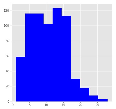
The distribution is similar to a lognormal with a median of 11 seasons. These statistics take into account only the number of seasons played by 2017 by current players, so the median score is clearly underestimated.
To get a more accurate value, we estimate the survival function using the lifelines library:
The library syntax is similar to scikit-learn and its fit / predict: by initiating KaplanMeierFitter, we then train the model on data. The fit method takes the career_length time interval and the observed vector as an argument.
Finally, when the model is trained, we can build a survival function for NHL players:
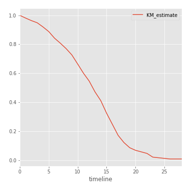
Each point on the chart is the probability that the player will play more than t seasons. As you can see, 80% of players overcome the milestone in 6 seasons, while a very small number of players manage to play more than 17 seasons in the NHL. Now more strictly:
Thus, 50% of NHL players will play more than 13 seasons, which is 2 seasons more than the initial estimate. Hockey players' chances to play more than 5 and 20 seasons are 88.8% and 6.9%, respectively. Great incentive for young players!
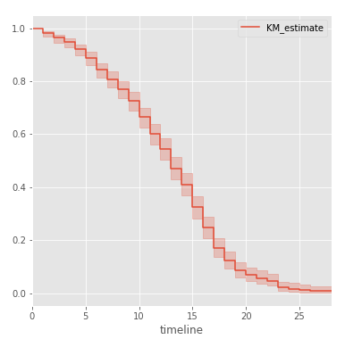
We can also derive the survival function, along with confidence intervals for probability:
Similarly, we construct the threat function using the Nelson-Aalen procedure:
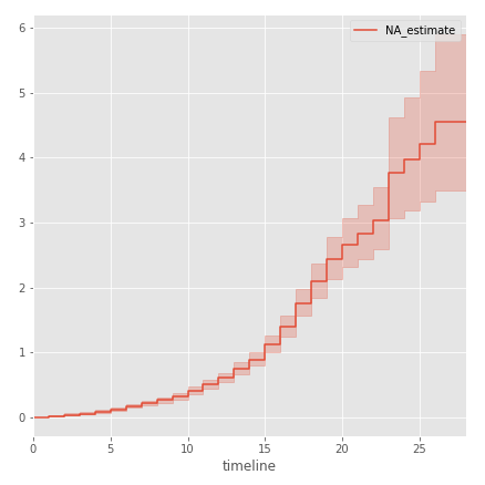
As can be seen on the graph, during the first 10 years the risk of an NHL player’s retirement at the end of the season is extremely small, but after the 10th season this risk is sharply increasing. In other words, spending 10 seasons in the NHL, the player will increasingly think about how to complete a career.
Now let's compare the length of the career of a defender and an NHL attacker. Initially, we assume that strikers play on average much longer than defenders, since they are often more popular among fans, so they often get long-term contracts. Also, with age, the players become slow, which hurts the most for defenders, who find it increasingly difficult to cope with brisk attackers.
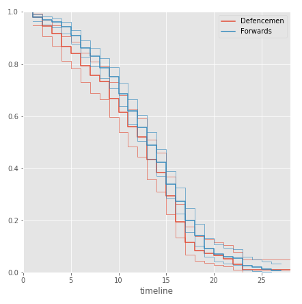
It seems that the length of the career defenders a little shorter than the attackers. To verify the accuracy of the output, we will conduct a statistical test based on the chi-square test:
So, at 10% level of significance, we reject the null hypothesis: the defenders do have a greater chance of completing their careers earlier than the attackers, while, as can be seen from the diagram, the difference increases towards the end of the career, which also confirms the earlier idea: behind the game and becoming less in demand.
Often we also have other factors that affect the duration of “life” that we would like to take into account. For this, a survival regression model was developed, which, like the classical linear regression, has a dependent variable and a set of factors.
Consider one of the popular approaches to estimating regression parameters — the additive Aalen model, which chose not the time intervals themselves as the dependent variable, but the values of the threat function calculated on their basis :
Let us turn to the implementation of the model. As factors of the model, we take the number of points, the position of the player, the date of the beginning of the career and the overall utility of the team (±):
Now that everything is ready, we will teach survival regression:
Let's try to estimate how many more seasons 2 players will play in the NHL: Derek Stepan, an attacker who started his career in 2010 and scored 310 points with a utility rating of +109 and compare it with the less successful NHL player - Klas Dalbek, who ended up in the NHL in 2014, scored 11 points with a utility rating of -12.
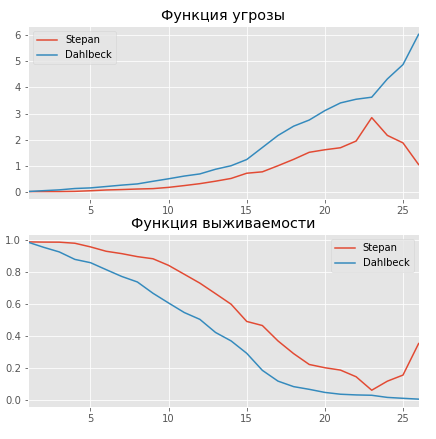
As expected, the more successful player has a longer career expectancy. So, Stepan has a chance to play more than 11 seasons - 80%, while Dalbek has only 55%. Also from the threat curve it can be seen that starting from season 13, the risk of completing a career for the next season increases dramatically, and at Dalbek it grows faster than Stepan.
To more strictly assess the quality of regression, we use the cross-validation procedure built into the lifelines library. At the same time, while working with censored data, we cannot use rms error and similar criteria as a quality metric, therefore the library uses a concordance index or a consent index, which is a generalization of the AUC-metric. Perform 5-step cross-validation:
The average accuracy for all iterations is 76.4% with a deviation of 2.7%, which indicates a fairly good quality of the algorithm.
When does this patient relapse? When will our client leave? Answers to such questions can be found using survival analysis, which can be used in all areas where the time interval from the “birth” to the “death” of an object is studied, or similar events: the period from the arrival of equipment to its failure, from the start of use services of the company and to abandon them, etc. Most often, these models are used in medicine, where it is necessary to assess the risk of death in a patient, which explains the name of the model, but they are also applicable in the manufacturing, banking and insurance sectors.
')
It is obvious that among the objects under consideration there will always be those for which the “death” (failure, occurrence of the insured event) has not yet occurred, and not taking them into account is a common mistake among analysts, since in this case they do not include the most relevant information in the sample and can artificially underestimate the time interval. To solve this problem, a survival analysis was developed, which assesses the potential “life expectancy” of observations with a “death” that has not yet occurred.
NHL Player Career Analysis
Data and Survival Curve
Above we talked about the application of this approach in medicine and economics, but now consider a less trivial example - the length of the career of NHL players. We all know that hockey is a very dynamic and unpredictable game, where you can, like Gordie Howe (26 seasons), play at the highest level for many years, or because of an unsuccessful collision you can finish your career after a couple of seasons. Therefore, we find out: how many seasons can a hockey player spend in the NHL and what factors influence the length of his career?
Let's look at the data already cleared and ready for analysis:
df.head(3) | Name | Position | Points | Balance | Career_start | Career_length | Observed |
|---|---|---|---|---|---|---|
| Olli Jokinen | F | 419 | -58 | 1997 | 18 | one |
| Kevyn adams | F | 72 | -14 | 1997 | eleven | one |
| Matt pettinger | F | 99 | -44 | 2000 | ten | one |
Data were collected on 688 NHL hockey players who have played since 1979 and played at least 20 matches, their position on the field, the number of points scored, team benefits (±), the start of a career in the NHL and its duration. The observed column indicates whether the player has completed his career, that is, players with a value of 0 are still in the league.
Let's look at the distribution of players by the number of seasons played:
The distribution is similar to a lognormal with a median of 11 seasons. These statistics take into account only the number of seasons played by 2017 by current players, so the median score is clearly underestimated.
To get a more accurate value, we estimate the survival function using the lifelines library:
from lifelines import KaplanMeierFitter kmf = KaplanMeierFitter() kmf.fit(df.career_length, event_observed = df.observed) Out:<lifelines.KaplanMeierFitter: fitted with 1808 observations, 340 censored> The library syntax is similar to scikit-learn and its fit / predict: by initiating KaplanMeierFitter, we then train the model on data. The fit method takes the career_length time interval and the observed vector as an argument.
Finally, when the model is trained, we can build a survival function for NHL players:
kmf.survival_function_.plot() Each point on the chart is the probability that the player will play more than t seasons. As you can see, 80% of players overcome the milestone in 6 seasons, while a very small number of players manage to play more than 17 seasons in the NHL. Now more strictly:
print(kmf.median_) print(kmf.survival_function_.KM_estimate[20]) print(kmf.survival_function_.KM_estimate[5]) Out:13.0 0.0685611305647 0.888063315225 Thus, 50% of NHL players will play more than 13 seasons, which is 2 seasons more than the initial estimate. Hockey players' chances to play more than 5 and 20 seasons are 88.8% and 6.9%, respectively. Great incentive for young players!
We can also derive the survival function, along with confidence intervals for probability:
kmf.plot() Similarly, we construct the threat function using the Nelson-Aalen procedure:
from lifelines import NelsonAalenFitter naf = NelsonAalenFitter() naf.fit(df.career_length,event_observed=df.observed) naf.plot() As can be seen on the graph, during the first 10 years the risk of an NHL player’s retirement at the end of the season is extremely small, but after the 10th season this risk is sharply increasing. In other words, spending 10 seasons in the NHL, the player will increasingly think about how to complete a career.
Comparison of attackers and defenders
Now let's compare the length of the career of a defender and an NHL attacker. Initially, we assume that strikers play on average much longer than defenders, since they are often more popular among fans, so they often get long-term contracts. Also, with age, the players become slow, which hurts the most for defenders, who find it increasingly difficult to cope with brisk attackers.
ax = plt.subplot(111) kmf.fit(df.career_length[df.Position == 'D'], event_observed=df.observed[df.Position == 'D'], label="Defencemen") kmf.plot(ax=ax, ci_force_lines=True) kmf.fit(df.career_length[df.Position == 'F'], event_observed=df.observed[df.Position == 'F'], label="Forwards") kmf.plot(ax=ax, ci_force_lines=True) plt.ylim(0,1); It seems that the length of the career defenders a little shorter than the attackers. To verify the accuracy of the output, we will conduct a statistical test based on the chi-square test:
from lifelines.statistics import logrank_test dem = (df["Position"] == "F") L = df.career_length O = df.observed results = logrank_test(L[dem], L[~dem], O[dem], O[~dem], alpha=.90 ) results.print_summary() Results t 0: -1 test: logrank alpha: 0.9 null distribution: chi squared df: 1 __ p-value ___|__ test statistic __|____ test result ____|__ is significant __ 0.05006 | 3.840 | Reject Null | True So, at 10% level of significance, we reject the null hypothesis: the defenders do have a greater chance of completing their careers earlier than the attackers, while, as can be seen from the diagram, the difference increases towards the end of the career, which also confirms the earlier idea: behind the game and becoming less in demand.
Survival regression
Often we also have other factors that affect the duration of “life” that we would like to take into account. For this, a survival regression model was developed, which, like the classical linear regression, has a dependent variable and a set of factors.
Consider one of the popular approaches to estimating regression parameters — the additive Aalen model, which chose not the time intervals themselves as the dependent variable, but the values of the threat function calculated on their basis :
Let us turn to the implementation of the model. As factors of the model, we take the number of points, the position of the player, the date of the beginning of the career and the overall utility of the team (±):
from lifelines import AalenAdditiveFitter import patsy # patsy, design # -1 , X = patsy.dmatrix('Position + Points + career_start + Balance -1', df, return_type='dataframe') aaf = AalenAdditiveFitter(coef_penalizer=1.0, fit_intercept=True) # penalizer, , ) Now that everything is ready, we will teach survival regression:
X['L'] = df['career_length'] X['O'] = df['observed'] # career_length observed aaf.fit(X, 'L', event_col='O') Let's try to estimate how many more seasons 2 players will play in the NHL: Derek Stepan, an attacker who started his career in 2010 and scored 310 points with a utility rating of +109 and compare it with the less successful NHL player - Klas Dalbek, who ended up in the NHL in 2014, scored 11 points with a utility rating of -12.
ix1 = (df['Position'] == 'F') & (df['Points'] == 360) & (df['career_start'] == 2010) & (df['Balance'] == +109) ix2 = (df['Position'] == 'D') & (df['Points'] == 11) & (df['career_start'] == 2014) & (df['Balance'] == -12) stepan = X.ix[ix1] dahlbeck = X.ix[ix2] ax = plt.subplot(2,1,1) aaf.predict_cumulative_hazard(oshie).plot(ax=ax) aaf.predict_cumulative_hazard(jones).plot(ax=ax) plt.legend(['Stepan', 'Dahlbeck']) plt.title(' ') ax = plt.subplot(2,1,2) aaf.predict_survival_function(oshie).plot(ax=ax); aaf.predict_survival_function(jones).plot(ax=ax); plt.legend(['Stepan', 'Dahlbeck']); As expected, the more successful player has a longer career expectancy. So, Stepan has a chance to play more than 11 seasons - 80%, while Dalbek has only 55%. Also from the threat curve it can be seen that starting from season 13, the risk of completing a career for the next season increases dramatically, and at Dalbek it grows faster than Stepan.
Cross validation
To more strictly assess the quality of regression, we use the cross-validation procedure built into the lifelines library. At the same time, while working with censored data, we cannot use rms error and similar criteria as a quality metric, therefore the library uses a concordance index or a consent index, which is a generalization of the AUC-metric. Perform 5-step cross-validation:
from lifelines.utils import k_fold_cross_validation score = k_fold_cross_validation(aaf, X, 'L', event_col='O', k=5) print (np.mean(score)) print (np.std(score)) Out:0.764216775131 0.0269169670161 The average accuracy for all iterations is 76.4% with a deviation of 2.7%, which indicates a fairly good quality of the algorithm.
Links
- Lifelines library documentation
- J.Klein, M.Moeschberger. Survival Analysis. Techniques for censored and truncated data is a book with many examples and datasets that can be accessed through the KMsurv package in R.
Source: https://habr.com/ru/post/333628/
All Articles