Remove "4D video" using a depth-sensor and Delaunay triangulation

Hi Habr! This is a note about a small hobby project that I did in my free time. I will tell you how to use simple algorithms to turn depth maps from depth sensors into a fun kind of content - dynamic 3D scenes (also called 4D video, volumetric capture or free-viewpoint video). My favorite part in this paper is the Delaunay triangulation algorithm, which allows you to turn sparse clouds of points into a dense polygonal mesh. I invite everyone who is interested in reading about algorithms, samopisnye bicycles in C ++ 11, and, of course, look at the three-dimensional seals.

For starters: this is what happens when using the RealSense R200: skfb.ly/6snzt (wait a few seconds to load the textures, and then use the mouse to rotate the scene). There is more under the cut!
Holders of limited rates, be careful. The article has a lot of different images and illustrations.

Disclaimer: in this article there will not be a word about artificial intelligence, blockchain or gravitational waves. It's just a small toy, which I wrote mostly to refresh C ++ and OpenGL. All expectations are formed, let's go!
')
Some time ago I got into the hands of a device with a 3D sensor, namely the Google Tango Development Kit tablet with the structured light technology. Naturally, my hands were itching to program something for this interesting device.

Just about the same time I first met a new kind of content - 4D video. By “4D video” I understand three-dimensional scenes that evolve over time in a non-trivial way, i.e. their behavior cannot be described by a simple model, such as skeletal animation or blendsheep. In short, something like this:



Such content seemed very interesting to me; I decided to experiment with it a bit and write my application to generate 4D videos. Of course, I do not have a studio and resources like Microsoft Research, and there is only one sensor, so the results will be much more modest. But that won't stop amateur programming, right? That I succeeded, I will tell in this article.



Most of the audience is undoubtedly familiar with 3D sensors. The most massive device in this category is the well-known Kinect, a very successful product from Microsoft. However, despite the relative prevalence, for many people, depth-sensors remain something outlandish. It will be useful for us to understand the principle of their work before starting to write applications.

With Google Tango and other structured light devices, everything is relatively clear. An infrared illuminator built into the device projects an irregular pattern of light points onto the scene, something like this picture:



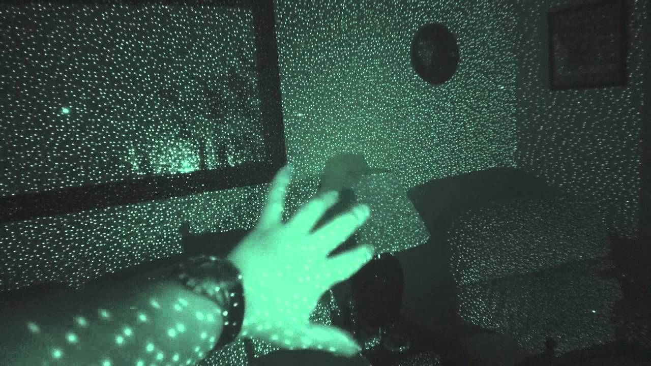
Then the special software turns the distortions of this pattern on the image from the IR camera (caused by the various shapes of objects) into a series of 3D measurements. For each spot of light in the picture, the algorithm restores the spatial coordinates, and at the output we get a 3D cloud of points. Inside, of course, everything is much more interesting, but this is a topic for a whole separate article.

Well, you need to check how it works in practice! For a couple of evenings, a simple grabber application for the Tango-tablet on Android was written on my knee, and here I have my very first dataset.


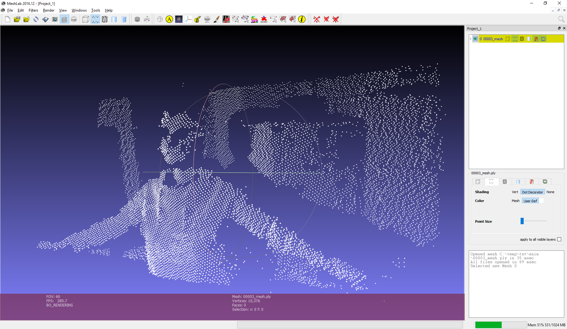
Although the first version of the grabber was very raw, the main thing was achieved: the coordinates of the points were recorded in a binary file. The screenshot shows what a cloud of points looks like from one frame in the Meshlab program.

Ok, point cloud is already interesting. However, the point cloud is a very “sparse” view of the scene, because the resolution of modern structured light sensors is rather low (usually around 100x100 pixels, plus or minus). And in general, in the world of computer graphics, a different representation of 3D objects and scenes, namely polygonal grids, or meshes, is much more familiar.

If you think about it, the task of getting a mesh through a cloud of points from a single 3D camera is quite simple, much simpler than arbitrary meshing in 3D. For this, we do not need any marching cubes or a reconstruction of Poisson . Recall that the points were obtained using a single IR camera and are naturally projected back onto the focal plane:



Now we can solve the problem in 2D, forgetting for a while about the Z-coordinate. To get polygons you only need to triangulate a set of points on a plane. Once this is done, we project the vertices back to 3D using the internal parameters of the IR camera and the known depth at each point. Triangulation will dictate the connectivity between the vertices, i.e. we interpret each triangle as a mesh face. Thus, on each frame you get a real 3D model of the scene, which can be rendered in OpenGL, opened in Blender, etc.

So, all that remains to be done is to find the triangulation for points on each frame. There are lots of ways to triangulate a set of points in 2D, and in fact any triangulation will give us some kind of mesh. But exactly one method is optimal for building a polygonal mesh - Delaunay triangulation.

This interesting construction has been mentioned many times on Habré, but I’ll still write a few words. All of us have seen Voronoi diagrams. The Voronoi diagram for a set of points S is such a partition of the plane into cells, where each cell contains all the points closest to one of the elements of S.




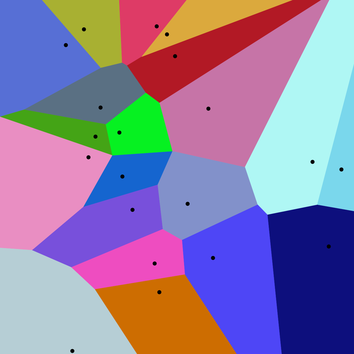
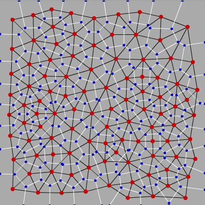
And Delaunay triangulation is such a triangulation, which in the sense of graph theory is dual to the Voronoi diagram:



Delone triangulations have many remarkable properties, but these two are especially interesting to us:

1. The circle described around any of the triangles does not contain points of the set, except for the vertices of the triangle itself.
2. Delaunay triangulation maximizes the minimum angle among all the angles of all triangles, thereby avoiding degenerate and “thin” triangles.

Property # 2 quite intuitively follows from # 1. Indeed, in order for the circumscribed circles to contain extraneous points, they must be as small as possible, and the radius of the circle for “thin” triangles (close to degenerate), on the contrary, is very large. Thus, the Delaunay triangulation maximizes the number of “good” triangles far from degenerate. And that means our mesh should look good.

No sooner said than done, we write Delaunay triangulation. There are many well-known algorithms, the simplest ones start somewhere with $$$O (n ^ 4)$. But once people have learned to count these triangulations as $$$O (nlogn)$, we just can not be slower!

As in many other similar problems, the algorithm is based on the principle of “divide and conquer”. We will sort the points by x and y coordinates, and then recursively generate and merge triangulations until we have one large graph. It is enough to show this piece of code so that it becomes clear what is happening here:

const uint16_t numRight = numPoints / 2, numLeft = numPoints - numRight; EdgeIdx lle; // CCW convex hull edge starting at the leftmost vertex of left triangulation EdgeIdx lre; // CW convex hull edge starting at the rightmost vertex of left triangulation EdgeIdx rle; // CCW convex hull edge starting at the leftmost vertex of right triangulation EdgeIdx rre; // CW convex hull edge starting at the rightmost vertex of right triangulation triangulateSubset(lIdx + numLeft, numRight, rle, rre); triangulateSubset(lIdx, numLeft, lle, lre); mergeTriangulations(lle, lre, rle, rre, le, re); 

In principle, everything can disperse.

Not really, because the fun begins in the mergeTriangulations function. Indeed, if we have divided our set in half a sufficient number of times, we are left with pieces of two or three points, with which we will somehow sort things out:



And then what?


In fact, too, nothing complicated. In each sheet of recursion we have already received a valid solution of the subtask. It remains to go up the stack, merging the left and right partitions into a single unit along the way. But this should be done carefully, because far from each method of merging will give us Delone triangulation at the output.

The algorithm of Gibas and Stolfi offers a very elegant solution to this problem. The idea is to use property # 1, which I mentioned above, but in order.
First, some notation; let's call the left triangulation L, and the right R. Then the edges belonging to the left triangulation will be called LL, since they begin and end at points of the left subset. The edges of the right triangulation are called RR, and the edges that we add between the left and right half are called LR, just like in the illustration:



As you can see, here we have already “started” starting triangles and edges in triangulation from as many as four triangles. All edges that were present in the previous step are marked as LL or RR, and all new edges are marked LR. The merging process at this step is not shown, since it is rather trivial and will not allow to show the features of the algorithm. But the next step will be more interesting, let's consider it. Here is our task before the start of the merger:



Note that the “outer” edges in the left and right half (such as 1-2, 2-5, 5-4, 6-8) form the convex hulls of their subset of points. It is clear that such edges always belong to the Delaunay triangulation, and indeed any triangulation. Note also that when merging two non-intersecting partitions, we will always need to add exactly two new edges in order to complete the convex hull of the unified set (roughly speaking, to “cover” the points with new edges from above and below). Great, we already have two new LR-edges! Choose one of them, the bottom one, and call it “base” (in the code - base).



Now we have to add the next edge adjacent to base, with one of its ends coinciding with the end of base, and the other end is a point from either L or R. Actually, we need to decide which of the two options is correct. Let's start on the right side. The first candidate will be a point associated with the right end of the base RR-edge with the smallest angle clockwise relative to the base. The next candidates in turn will be the points R connected to the right vertex of the base RR-edges with an increasing angle value relative to the base, as shown in the illustration:



Now for each candidate you need to check two conditions:

1. The angle between the base and the candidate should not exceed 180 degrees (we are only interested in points that are “higher” than the base).
2. The circle described around the base and the candidate point must not contain the next candidate point.

Depending on the configuration of the vertices, there may be several options:

• There was a candidate point that satisfies both criteria. Great, this will be our choice for the right side.
• If requirement # 1 is not fulfilled (angle <180 degrees), then we have already reached the “top”, and there is no longer a need to choose points from the right side. We consider only the left triangulation.
• The most interesting case is the condition # 1, but not # 2 (see illustration). In this case, we need to remove the RR-edge that connects the base with the candidate point and repeat the search again.

Naturally, the process for the left half is completely symmetrical.



Thus, with each addition of a new LR edge, we select a candidate point from the left and right half. If neither there nor there was a suitable point, then we have completed the merger and need to go further up the stack. If there is one point (only on the left or just on the right), we add an LR-edge with an end in it. If points were found on both sides, we repeat the test with a circle: we build the circumscribed circle around the base and the candidate points from L and R. We select the point whose circumference does not contain the candidate from the opposite half. Fact: such a point will always be unique, unless the four vertices form a rectangle. In this case, you can choose any of the options.



In this example, we select a candidate from L, because the corresponding circle does not contain a candidate point from R.

After a new LR edge is added, it becomes a new “base” (base). Repeat base update until we reach the top edge of the convex hull:


It turns out that if our algorithm accurately follows the described rules, then after merging the left and right half we get a valid Delaunay triangulation for L∪R.

"I found this truly miraculous proof, but the fields of this book are too narrow for him." In fact, if you're wondering where all the statements came from, for example about the need to remove edges, I recommend exploring the work of Gibas and Stolfi , key lemmas numbered 9.2, 9.3, 9.4, 8.3.

Well, now let's put everything together and see what happens:



This is a visualization of the work of the algorithm, which I got. Here, the base edge is marked orange, the LL candidate is green, the RR candidate is blue. Red marked edges that do not meet criterion # 2 and will be deleted.

While the description of the algorithm is still fresh in memory, it is very easy to understand that it is really executed in $$$O (nlogn)$. Indeed, we have order $$$logn$merge operations; even if on each of them we are forced to remove and rebuild all edges in general, the number of actions will still be of the order $$$n$(since it is a triangulation, and not an arbitrary graph, the number of edges is linear with respect to the number of points). In fact, on most real-world tasks, speed is better than $$$O (nlogn)$and close to linear; we need some especially patient dataset to force the algorithm to rebuild triangulation from scratch at each merging stage.

Another remark is that it is easy to obtain from the obtained triangulation both the convex hull and the Voronoi diagram for the corresponding set of points. Pleasant bonus.

It is interesting to say a few words about the data structure that I used to work with the graph. Usually, graphs are represented as lists or adjacency matrices, but in this problem we are interested not only in connectivity, but also in some geometric properties of the graph. Here's what I got:

 struct TriEdge { uint16_t origPnt; // index of edge's origin point EdgeIdx symEdge; // index of pair edge, with same endpoints and opposite direction EdgeIdx nextCcwEdge; // next counterclockwise (CCW) edge around the origin EdgeIdx prevCcwEdge; // previous CCW edge around the origin (or next CW edge) }; 

This is in some way a trimmed version of the structure that Gibas and Stolfi offer. As they say, all ingenious is simple. For each edge we store the point from which it “goes out” (origin), the index of its pair edge directed in the opposite direction, as well as the indices of the next and previous edge “around” the origin point. In fact, we get a doubly linked list, but since we maintain the relative position of the edges around their ends, many steps of the algorithm are simply encoded elementarily.

In some other works it is proposed to store not the edges, but triangles at once. I tried to experiment with this option, and I can say that the amount of code grows many times, because it is necessary to introduce numerous crutches for special cases (degenerate triangles, points at infinity, etc.). And although this option has a potential advantage in terms of memory usage, I strongly recommend using double-linked edge lists. Working with them at times is more pleasant.

I think from now on you can stop pretending that someone is interested in the details of the implementation of the algorithm. You can just relax and pozalipat these wonderful animations.



How about a regular grid?



Here the points were successfully divided into subsets and did not have to remove any edges at all. But this is not always the case.



Already more interesting. The number of points on the lattice side became odd and because of this, the algorithm is forced to make quite a few corrections. How about a circle of dots?



Interesting! But I like it better with a dot in the center:



I think by this point the article contains a sufficient number of GIF-animations. In order for readers with traffic restrictions to have at least a little bit of Internet after downloading this article, I uploaded the rest of the animations to video hosting.

It is recommended to stick in 1080p and 60fps, this is the original video resolution. And it is better to expand to the full screen, otherwise the edges of the graph are alias.



I realize that these videos are far from being interesting to everyone, but they have the same effect on me as the “pipeline” screensaver in older versions of Windows. Hard to break away.



These animations were the main reason why the article was written for so long. Note to self: next time it’s dangerous to do debugger and traces, it’s dangerous to do debug visualizations :) If someone wants to look at the work of the algorithm on other configurations of points, write in the comments, I’ll be happy to generate more animations.



Having fun with visualization was fun, but it's time to remember why the algorithm was originally created. We were going to generate a polygon mesh from the data from the depth-sensor. Well, let's take a cloud of points from the sensor, project it onto the camera plane and launch the triangulation algorithm.

(Do not ask me how much this video was rendered. Poor ffmpeg.)

So, great! Although at this stage we only have a graph of points and edges, we can generate an array of triangles from it in an elementary way. It remains only to filter ugly polygons stretched along the Z-coordinate, which appear on the borders of the objects and make a simple OpenGL player:



Here you can clearly see that the first version of the grabber was very raw: half the frames did not have time to register, because of this, the picture freezes. In short, hardly a directing masterpiece. But it does not matter - the algorithms are finally alive! For me, it was a real “train arrival”!

After that, I shot a couple more clips, I uploaded them to the Sketchfab resource in the timeframe animation format, it seems to me more interesting.

Dataset # 2 in WebGL
Dataset # 3 in WebGL

Well, the pipeline has earned and it has become clear that further development limits the possibilities of iron. Indeed, the Tango tablet allows you to shoot only at a very low frame rate (5 fps), but the main idea was to capture the dynamic nature of the scenes. There is another significant limitation: in Tango, RGB and IR cameras are not synchronized, that is, frames are received at different points in time. This is not critical for, say, scanning static objects, since Tango SDK allows you to find the conversion between the RGB and IR positions for adjacent frames using the built-in tracking based on the high-frequency accelerometer and fisheye camera. But with moving objects, this does not help at all, and for me the lack of synchronization meant that the mesh would not be able to pull the texture.

Fortunately, I had another device - Intel RealSense R200 . Miraculously, the R200 does not have both disadvantages, since It develops up to 60 (!) fps and has excellent synchronization of all its cameras. So I decided to write a grabber application for the R200 (this time in C ++ , not Java) and continue the experiments.

Immediately it became clear that there was a small problem with my pipeline. With the increased resolution and high shooting frequency that the R200 allows, there was already not enough performance to generate a mesh on every frame in realtime. Profiling showed that the bottleneck is of course triangulation. The original version was written quite “relaxedly”, with dynamic memory allocation, using STL, etc. In addition, the first version worked with coordinates of type float, although in my task the points always have integer coordinates (positions in pixels in the picture). So it is not surprising that, from the asymptotic point of view, a good algorithm worked on my laptop for up to 30 milliseconds on a test frame from Tango (about 12,000 points). The potential for acceleration was obvious and I enthusiastically sat down to optimize. Events developed something like this:

• First of all, floating-point numbers set off for the altar of speed. All algorithms (where possible) switched to integer calculations.
• The second in line was the dynamic allocation of memory. Now all the memory for the algorithm was allocated once, “for the worst case,” and then reused. Not the most effective solution in terms of memory consumption (in the spirit of ACM ICPC), but this gave a significant acceleration.
• A remarkable test was found on the project site for a numerical simulation of earthquakes to find a point inside the circumscribed circle of a triangle:
  
  Here is its implementation:
  
  

   FORCE_INLINE bool inCircle(int x1, int y1, int x2, int y2, int x3, int y3, int px, int py) { // reduce the computational complexity by substracting the last row of the matrix // ref: https://www.cs.cmu.edu/~quake/robust.html const int p1p_x = x1 - px; const int p1p_y = y1 - py; const int p2p_x = x2 - px; const int p2p_y = y2 - py; const int p3p_x = x3 - px; const int p3p_y = y3 - py; const int64_t p1p = p1p_x * p1p_x + p1p_y * p1p_y; const int64_t p2p = p2p_x * p2p_x + p2p_y * p2p_y; const int64_t p3p = p3p_x * p3p_x + p3p_y * p3p_y; // determinant of matrix, see paper for the reference const int64_t res = p1p_x * (p2p_y * p3p - p2p * p3p_y) - p1p_y * (p2p_x * p3p - p2p * p3p_x) + p1p * (p2p_x * p3p_y - p2p_y * p3p_x); assert(std::abs(res) < std::numeric_limits<int64>::max() / 100); return res < 0; } 

These three events gave a very significant acceleration, from 30000+ to 6100 microseconds per frame. But it was possible to accelerate more:

• Made some small functions __forceinline, 6100 -> 5700 microseconds, a rare case when the compiler did not guess.
• Removed #pragma pack (push, 1) for TriEdge structure. And why did I decide that packing will be faster? 5700 -> 4800 microseconds.
• Replaced std :: sort for points with self-written sorting, similar to radix. 4800-> 3700 microseconds.

Total it turned out to speed up the code almost 10 times, and I think this is not the limit. By the way, I was not too lazy to collect code for Android, and on a similar ARM task, the Tango processor worked for about 10 milliseconds per frame, i.e. 100 fps! In short, it turned out even a little overkill, but if someone needs a very fast “integral” Delone triangulation, then welcome to the repository.

Now my algorithms were ready for the R200, and here is the first dataset I took:



It was naturally followed by others. I will not attach the video of my OpenGL viewer, I think it's more interesting to look directly at Sketchfab: skfb.ly/6s6Ar

It is recommended to open no more than one clip at a time, since Sketchfab loads all dataset frames into memory at once, and in general the viewer is not very fast. By the way, here is the promised 4D cat (Vasya):

• skfb.ly/6s6AC
• skfb.ly/6s6AJ

Dog Totoshka was not very happy that they shine a laser at him. But he had no choice:

• skfb.ly/6s6AP
• skfb.ly/6s6BH

There are a few more clips in my account on Sketchfab. Of course, the quality of the models can be improved if you carefully filter the noise from the sensor, you can reduce the number of points, so that the player on the site does not brake so much, etc. But as they say, there is no limit to perfection; I already spent a lot of time on this pet project.

And in general, given the aggressive offensive of AR and VR, I am sure that the developers will not devour attention to these tasks. More volumetric content like CG is found on the web:


and shot in real life:


Agree, it looks very impressive! In general, there is no need to worry about the future of free-viewpoint video.

Finally, all the code written for this project is available on Github under a free license. Although the generated 4D videos were hardly impressive, the algorithms still have the potential for further use and development.
The main advantage of the approach described in the article is that the 3D scene is generated on the fly in realtime, in the player itself. Because of this, in compressed form, videos can take up very little space, in fact almost as much as a similar traditional video.

Indeed, the usual RGB video we need only for textures, and the 3D coordinates of the points can be saved as sparse depth maps and also encoded into a video file, already in grayscale. Thus, for rendering one frame in 3D, we need only frames from two videos and some metadata (camera parameters, etc.). Based on this, you can make a cool application, say, Skype in augmented reality. The interlocutor removes the depth-camera, and your iPhone renders the talking 3D head in real time using ARKit. Almost like holograms from Star Wars.

There is another option that can be useful to users of Tango. The fact is that Tango SDK provides data in the form of point clouds in 3D (as I described above), while for many algorithms you want to have a dense depth map (depth map). The most common way to obtain it is to project points onto the focal plane and interpolate the depth values ​​between adjacent points where it is known. So the combination of Delaunay + OpenGL triangulation allows you to do this interpolation accurately and efficiently. Due to the fact that rasterization occurs on the GPU, you can generate depth maps in high resolution, even on a smartphone.

But this is all the lyrics. So far, I'm just very glad that I finished the article. If you have any thoughts or feedback, I suggest to discuss in the comments.

Image credits

• Voronoi diagram
• Voronoi faces
• Voronoi giraffe
• Voronoi-Delaunay duality
• Algorithm