Is it possible to leave Klintsy? (data mining of blablacar.ru)
Parsing blablacar.ru website and analyzing passenger traffic from Klintsy, Bryansk region using the R programming language.

Prehistory
By the will of various circumstances, downshift in a small town of the Bryansk region (Klintsy). I live, I work, I am interested in cultural rest. "Where can I go here?" - I ask the locals. "It is best to go to the station for tickets," clinch benevolently advise.
I liked the idea, and decided to take one-two-day trips as an escape from worries, choosing Blablakar for this purpose (it’s more economical to pick up the travel time, you can talk with the driver, more choice of routes).
In order to better present: where, when, how and for how much you can leave Klintsy, he did a little research. Results, algorithm, scripts and data are shared in this article.
R libraries
The following R libraries were used for the study:
- rvest, Rselenium - data parsing;
- dplyr, tidyr - data manipulation;
- ggplot2, ggmap, grid, gridExtra - visualization;
- forecast, zoo - work with time series;
- aret, xgboost, mlr - machine learning.
Data acquisition
It was not possible to collect data from the site using standard R tools (rvest library). Blablakar works on JS, which forms dynamic pages depending on the user's request, and the rvest functions do not support them.
Since I am familiar with web technologies to the extent that I did, I didn’t understand where and what was on the server and how it tightened up, but chose a simpler, as it seemed to me, solution.
I installed a Rselenium server on my machine, launched Google Chrome through it, which formed the necessary page and saved the output. Further the page without problems was parsed by R.
Blablakar provides data in just two months (713 trips), so this scheme worked fine (since the third, crunching with crutches, the server started up). However, I am not sure that the algorithm is suitable for parsing more pages - too much time and resources are leaving, many bottlenecks.
#### #### # mnth <- 5:7 # days <- seq(1, 31, 1) # url.t <- c() urls <- c() for(i in mnth){ for(j in days){ url <- paste0("https://www.blablacar.ru/poisk-poputchikov/klintcy/#?db=", j, "/", i, "/2017&fn=%D0%9A%D0%BB%D0%B8%D0%BD%D1%86%D1%8B,+%D0%91%D1%80%D1%8F%D0%BD%D1%81%D0%BA%D0%B0%D1%8F+%D0%BE%D0%B1%D0%BB%D0%B0%D1%81%D1%82%D1%8C&fc=52.756616%7C32.256669&fcc=RU&fp=0&tn=&sort=trip_date&order=asc&radius=15&limit=100") url.t <- c(url.t, url) } urls <- c(urls, url.t) url.t <- c() } # urls <- urls[11:74] urls <- urls[-52] # 31 #### #### # blblcars <- data.frame(Name = character(), Age = character(), Date = character(), Time = character(), City = character(), Price = character(), stringsAsFactors = FALSE) # RSelenium rD <- rsDriver( browser = c("chrome")) remDr <- rD$client for (j in urls) { # remDr$navigate(j) # 3 , Sys.sleep(3) # html <- remDr$getPageSource() html <- read_html(html[[1]]) # names <- html_nodes(html, ".ProfileCard-info--name") names.i <- c() if (length(names) == 0) { names.i <- NA } else { for (i in 1:length(names)) { names.i[i] <- gsub(".*\n |\n.*", "", names[[i]]) } } # age <- html_nodes(html, ".u-truncate+ .ProfileCard-info") age.i <- c() if (length(age) == 0) { age.i <- NA } else { for (i in 1:length(age)) { age.i[i] <- gsub(".*: |<br/>.*", "", age[[i]]) } } # date <- html_nodes(html, ".time") date.i <- c() if (length(date) == 0) { date.i <- NA } else { for (i in 1:length(date)) { date.i[i] <- gsub(".*content=\"|\">.*", "", date[[i]]) } } # time <- html_nodes(html, ".time") time.i <- c() if (length(time) == 0) { time.i <- NA } else { for (i in 1:length(time)) { time.i[i] <- gsub(".* - |\n.*", "", time[[i]]) } } # price <- html_nodes(html, ".price") price.i <- c() if (length(price) == 0) { price.i <- NA } else { for (i in 1:length(price)) { price.i[i] <- gsub(".*<span class=\"\">\n|\n.*", "", price[[i]]) } } # city <- html_nodes(html, ".trip-roads-stop~ .trip-roads-stop") city.i <- c() if (length(city) == 0) { city.i <- NA } else { for (i in 1:length(city)) { city.i[i] <- gsub("<span class=\"trip-roads-stop\">|</span>", "", city[[i]]) } } # blblcars.t <- data.frame(Name = names.i, Age = age.i, Date = date.i, Time = time.i, City = city.i, Price = price.i, stringsAsFactors = FALSE) # blblcars <- rbind(blblcars, blblcars.t) } # RSelenium remDr$close() # save(blblcars, file = "data/blblcars") Traffic dynamics and prediction
#### #### # load("data/blblcars") # blblcars$Age <- as.integer(blblcars$Age) blblcars$Price <- as.integer(gsub("[^0-9]", "", blblcars$Price)) blblcars$hours <- as.integer(gsub(":..", "", blblcars$Time)) blblcars$days <- weekdays(as.Date(blblcars$Date)) On average, 10 cars a day leave Klintsy, the maximum is 35. Traffic is growing. What influences the positive dynamics - the holiday season, more favorable road conditions in the summer, the long-term growth of the service audience - it's hard to say for sure. We need data for at least a couple of years.
#### #### # row.names(blblcars)[is.na(blblcars$Price)] 2017-06-03 - blblcars$Date[214] <- "2017-06-03" # , # bl.date <- blblcars %>% count(Date) bl.date$n[bl.date$Date == "2017-06-03"] <- 0 bl.date$Date <- as.Date(bl.date$Date) bl.date <- bl.date %>% filter(Date != "2017-07-12") # Min. 1st Qu. Median Mean 3rd Qu. Max. # 0.00 8.00 10.00 11.48 13.00 35.00 summary(bl.date$n) #### " " #### ggplot(bl.date, aes(x = Date, y = n))+ geom_line()+ geom_smooth()+ labs(title = " ", subtitle = " . blablacar.ru 11 11 2017 .", caption = ": blablacar.ru silentio.su", x = "", y = " ")+ theme(legend.position = "none", axis.text.x = element_text(size = 14), axis.title.x = element_text(size = 14), axis.text.y = element_text(size = 14), axis.title.y = element_text(size = 14), title = element_text(size = 14)) 
Predicting traffic for the next week or month is also problematic. Tested several models, but the accuracy of predictions leaves much to be desired.
#### #### bl.arima <- zoo(bl.date$n, bl.date$Date) model.arima <- auto.arima(bl.arima) predic.ar <- forecast(model.arima, h = 14) plot(predic.ar, type = "line", main = " ") title(main = " ", xlab = "ARIMA(2,1,1), 12-25 2017 .", ylab = " ") grid.text(": blablacar.ru silentio.su", x = 0.98, y = 0.02, just = c("right", "bottom"), gp = gpar(fontsize = 14, col = "dimgrey")) 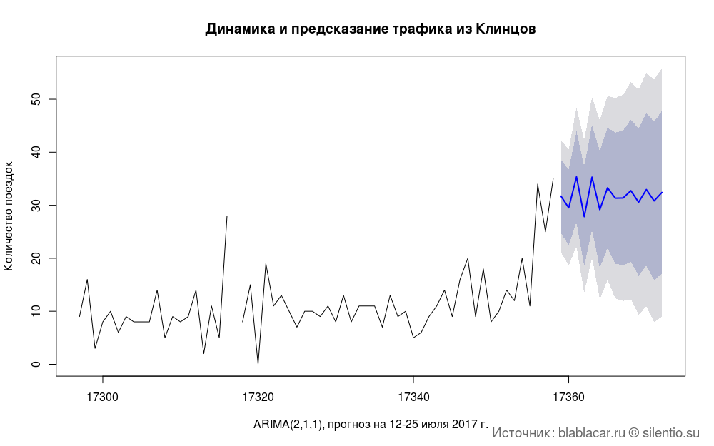
Most popular destinations
For two months, cars from Klintsy were sent to 59 different cities. However, there are few main directions: Bryansk (40% of all trips), Moscow (18%), cities of the Bryansk region, Gomel (border town in Belarus, regional center), Oryol, Smolensk - 88% of all trips.
#### #### bl.city <- blblcars %>% count(City) bl.city$percents <- round(bl.city$n/sum(bl.city$n)*100, digits = 2) bl.city <- bl.city %>% arrange(desc(n)) # 59 length(unique(bl.city$City)) #### "-10 . blablacar.ru" #### ggplot(bl.city[1:10,], aes(x = reorder(City, n), y = percents, fill = percents))+ geom_bar(stat = "identity")+ coord_flip()+ geom_label(aes(label = paste0(percents, "%")), size = 5, colour = "white", hjust = 1)+ labs(title = " ", subtitle = "-10 . blablacar.ru", caption = ": blablacar.ru silentio.su", x = "", y = "% ")+ theme(legend.position = "none", axis.text.x = element_text(size = 14), axis.title.x = element_text(size = 14), axis.text.y = element_text(size = 14), axis.title.y = element_text(size = 14), title = element_text(size = 14)) 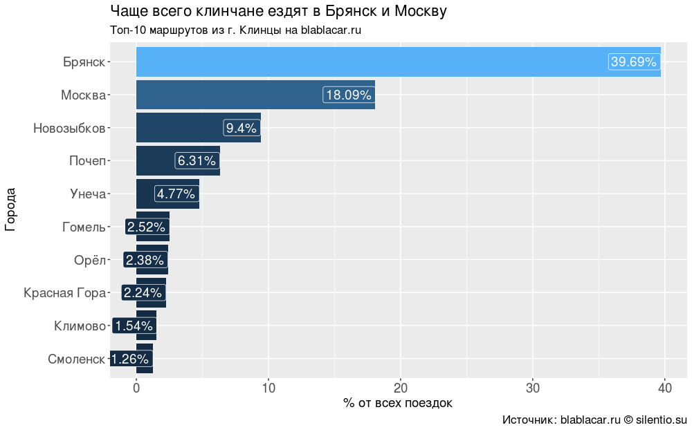
If you put the destination on the map, you get an almost perfect circle with a center in Klintsy and a radius of 1000-1200 km, dense in the center and discharged closer to the periphery. The arc Klintsy-Bryansk-Kaluga-Moscow is also clearly visible.
#### . blablacar.ru #### # bl.city <- na.omit(bl.city) geo <- geocode(bl.city$City) bl.city <- cbind(bl.city, as.data.frame(geo)) map <- get_map(location = "Klintsy", maptype = "terrain", zoom = 4) ggmap(map)+ geom_point(data = bl.city, aes(x = lon, y = lat, size = percents), alpha = 1, colour = "red")+ labs(title = " . blablacar.ru", caption = ": blablacar.ru silentio.su", x = " ", y = " ", size = "% :")+ theme(legend.position = "left", legend.text = element_text(size = 12), axis.text.x = element_text(size = 8), axis.title.x = element_text(size = 8), axis.text.y = element_text(size = 8), axis.title.y = element_text(size = 8), title = element_text(size = 14)) 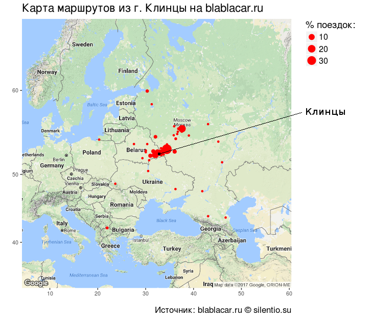
That is, mainly clinchans travel around the place, regularly travel to nearby regional centers and to the MSC.
Fare
The fare for all drivers, grouped in directions, is about the same: about 100 p. - in the region, an average of 280 p. - Bryansk, 900 p. - Moscow. It is somewhere around 25% cheaper than regular carriers.
The biggest price range is for tickets to Orel (from 350 to 600 rubles) and Smolensk (from 450 to 650 rubles).
#### -10 #### bl.price.top <- blblcars %>% filter(City %in% unique(bl.city$City[1:10])) %>% select(City, Price) bl.price.top <- full_join(bl.price.top, bl.price.top %>% group_by(City) %>% summarise(mean = mean(Price)) ) bl.price.top$mean <- round(bl.price.top$mean, digits = 0) bl.price.top$mean <- paste0(bl.price.top$mean, " .") bl.price.top <- bl.price.top %>% unite(City, c(City, mean), sep = ", ") #### " " #### ggplot(bl.price.top, aes(x = reorder(City, Price), y = Price))+ stat_summary(geom = "line", group = 1, fun.data = "mean_cl_boot", size = 1, colour = "blue")+ stat_summary(fun.data = "mean_cl_boot", colour = "red", size = 1)+ labs(title = " - ", subtitle = " . blablacar.ru (-10 )", caption = ": blablacar.ru silentio.su", x = " ", y = " , .")+ theme(legend.position = "none", legend.text = element_text(size = 14), axis.text.x = element_text(size = 14, angle = 90), axis.title.x = element_text(size = 14), axis.text.y = element_text(size = 14), axis.title.y = element_text(size = 14), title = element_text(size = 14)) 
Oddly enough, the price of the trip does not always depend on the distance. The most expensive trip from Klintsy to the South and the Caucasus is 1500-2300 r. For similar distances in the direction of Europe ask two times less.
#### #### bl.price <- blblcars %>% select(City, Price) %>% group_by(City) %>% summarise(price = mean(Price)) bl.price$price <- round(bl.price$price, digits = 0) bl.price <- bl.price %>% arrange(desc(price)) #### "-10 . blablacar.ru" #### ggplot(bl.price[1:10,], aes(x = reorder(City, price), y = price, fill = price))+ geom_bar(stat = "identity")+ coord_flip()+ geom_label(aes(label = paste0(price, " .")), size = 5, colour = "white", hjust = 1)+ labs(title = " ", subtitle = "-10 . blablacar.ru", caption = ": blablacar.ru silentio.su", x = "", y = " , .")+ theme(legend.position = "none", axis.text.x = element_text(size = 14), axis.title.x = element_text(size = 14), axis.text.y = element_text(size = 14), axis.title.y = element_text(size = 14), title = element_text(size = 14)) 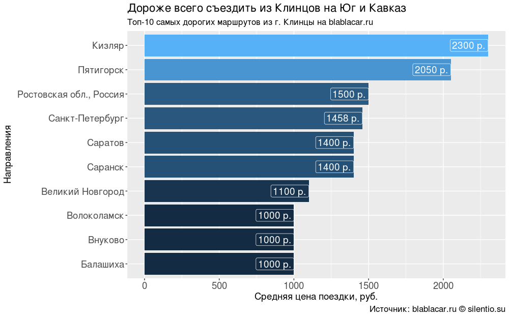
Driver analysis
I was interested in the motivation of drivers. Why do they charge passengers? Are among them those who use the service for commercial gain?
54% of drivers for two months only once used the service. The rest go with a frequency of 1 time per month to 1 time per week, probably on business cases - passengers are taken in order to reduce travel expenses.
I found only one person, who, most likely (but this is not accurate), is engaged in commercial carrying (route taxi, Novozybkov – Klintsy – Moscow route, every three days).
#### #### drivers <- blblcars %>% select(Name, Age) drivers$Age <- paste0(": ", drivers$Age) drivers <- drivers %>% unite(Name, c(Name, Age), sep = ", ") drivers <- drivers %>% count(Name) drivers$percents <- round(drivers$n/sum(drivers$n)*100, digits = 2) drivers <- arrange(drivers, desc(n)) drivers$per.month <- round(drivers$n/2, digits = 0) summary(as.factor(drivers$n))/sum(drivers$n)*100 #### " " #### ggplot(drivers[1:10,], aes(x = reorder(Name, n), y = percents, fill = percents))+ geom_bar(stat = "identity")+ coord_flip()+ geom_label(aes(label = paste0(per.month, " ./")), size = 5, colour = "white", hjust = 1)+ labs(title = " ", subtitle = "-10 . blablacar.ru", caption = ": blablacar.ru silentio.su", x = "", y = " ")+ theme(legend.position = "none", axis.text.x = element_text(size = 14), axis.title.x = element_text(size = 14), axis.text.y = element_text(size = 14), axis.title.y = element_text(size = 14), title = element_text(size = 14)) 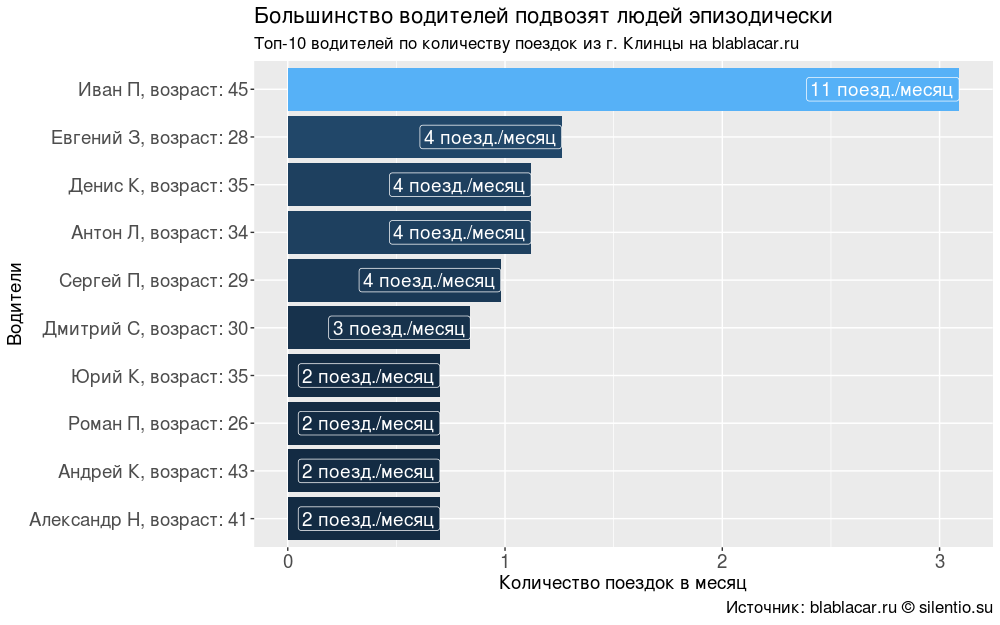
Departure time
The easiest way to leave Klintsy is from 16:00 to 19:00. Cars go to Moscow at night, at about nine in the evening.
#### -10 #### bl.hours <- blblcars %>% group_by(City) %>% count(hours) bl.hours <- ungroup(bl.hours) # for (i in unique(bl.hours$City)) { for (j in seq(0, 23, 1)) { if (!j %in% bl.hours$hours[bl.hours$City == i]) { bl.hours <- rbind(bl.hours, data.frame(City = i, hours = j, n = 0)) } } } # -10 bl.hours <- bl.hours %>% filter(City %in% bl.city$City[1:10]) bl.hours$percents <- round(bl.hours$n/sum(bl.hours$n)*100, digits = 2) #### " . blablacar.ru " #### ggplot(bl.hours, aes(x = hours, y = percents, fill = City))+ geom_bar(stat = "identity")+ labs(title = " 16:00 19:00", subtitle = " . blablacar.ru ", caption = ": blablacar.ru silentio.su", x = " ( )", y = "% ( -10)", fill = ":")+ theme(legend.position = "right", legend.text = element_text(size = 12), axis.text.x = element_text(size = 14), axis.title.x = element_text(size = 14), axis.text.y = element_text(size = 14), axis.title.y = element_text(size = 14), title = element_text(size = 14)) 
Most often, people leave the city on Tuesday, Friday and Sunday.
#### -10 #### bl.days <- blblcars %>% group_by(City) %>% count(days) bl.days <- ungroup(bl.days) # for (i in unique(bl.days$City)) { for (j in unique(bl.days$days)) { if (!j %in% bl.days$days[bl.days$City == i]) { bl.days <- rbind(bl.days, data.frame(City = i, days = j, n = 0)) } } } # -10 bl.days <- bl.days %>% filter(City %in% bl.city$City[1:10]) bl.days$percents <- round(bl.days$n/sum(bl.days$n)*100, digits = 2) # bl.days$days <- as.factor(bl.days$days) bl.days$days <- factor(bl.days$days, levels = c("", "", "", "", "", "", "")) #### " . blablacar.ru " #### ggplot(bl.days, aes(x = days, y = percents, fill = City))+ geom_bar(stat = "identity")+ labs(title = " , ", subtitle = " . blablacar.ru ", caption = ": blablacar.ru silentio.su", x = " ", y = "% ( -10)", fill = ":")+ theme(legend.position = "right", legend.text = element_text(size = 12), axis.text.x = element_text(size = 14), axis.title.x = element_text(size = 14), axis.text.y = element_text(size = 14), axis.title.y = element_text(size = 14), title = element_text(size = 14)) 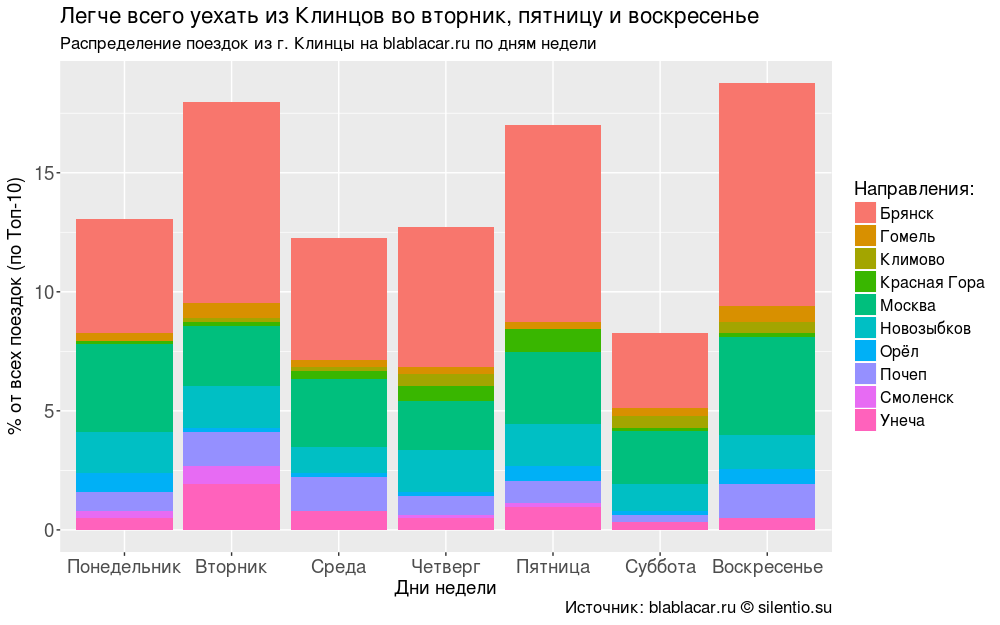
Conclusion
According to the results of the study, I made a schedule that explains where, when and for how much you can most likely leave if such a desire arises.
#### #### tbls <- blblcars %>% filter(City %in% bl.city$City[1:10]) %>% group_by(City) %>% select(City, days, Time, Price) # tbls <- full_join(tbls, tbls %>% summarise(mean.price = round(mean(Price), digits = 0)), by = "City" ) tbls <- tbls %>% select(-Price) # tbls <- full_join(tbls, tbls %>% count(days) %>% top_n(1, n), by = "City") for (i in unique(tbls$City)) { tbls$days.y[tbls$City == i] <- paste0(unique(tbls$days.y[tbls$City == i]), collapse = ", ") } tbls <- tbls %>% select(-c(days.x, n)) # tbls <- full_join(tbls, tbls %>% count(Time) %>% top_n(1, n), by = "City") for (i in unique(tbls$City)) { tbls$Time.y[tbls$City == i] <- paste0(unique(tbls$Time.y[tbls$City == i]), collapse = ", ") } tbls <- tbls %>% select(-c(Time.x, n)) tbls <- ungroup(tbls) tbls <- unique(tbls) tbls <- tbls[c("City", "days.y", "Time.y", "mean.price")] colnames(tbls) <- c(" ", " ", " ", " ") tbls <- tbls %>% arrange(` `) write.csv(tbls, file = "data/tbls.csv", row.names = F) 
I also trained in the xgboost algorithm, which predicts the most likely route based on the day of the week and departure time.
The most informative sign was the hour of departure. In the late night, the model consistently advises to go to Novozybkov, in the afternoon - to Bryansk, in the evening - to Moscow. Trips to other cities xgboost finds unlikely.
#### XGBOOST #### # df <- read.csv("data/ - .csv", stringsAsFactors = F) df <- df %>% select(c(City, Time, days)) df <- df %>% separate(Time, c("hours", "minutes"), sep = ":") df$days <- as.factor(df$days) levels(df$days) <- c("7", "2", "1", "5", "3", "6", "4") df[,2:4] <- apply(df[,2:4], 2, function(x) as.numeric(x)) top10 <- df %>% count(City) %>% arrange(desc(n)) top10 <- top10$City[1:10] df <- df %>% filter(City %in% top10) df <- na.omit(df) # df$class <- as.numeric(as.factor(df$City))-1 City.class <- df %>% select(City, class) City.class <- unique(City.class) df <- df[,-1] # train test # 1/3 indexes <- createDataPartition(df$class, times = 1, p = 0.7, list = F) train <- df[indexes,] test <- df[-indexes,] # y.train <- train$class # train.m <- data.matrix(train[,-4]) train.m <- xgb.DMatrix(train.m, label = y.train) # Stopping. Best iteration: # [15] train-merror:0.425361+0.010171 # test-merror:0.504626+0.035449 model <- xgb.cv(data = train.m, nfold = 4, eta = 0.03, nrounds = 2000, num_class = 10, objective = "multi:softmax", early_stopping_round = 200) # # train$class <- as.factor(train$class) traintask <- makeClassifTask(data = train, target = "class") lrn <- makeLearner("classif.xgboost", predict.type = "response") lrn$par.vals <- list(objective = "multi:softmax", eval_metric = "merror", nrounds = 15, eta = 0.03) params <- makeParamSet(makeDiscreteParam("booster", values = c("gbtree", "gblinear")), makeIntegerParam("max_depth", lower = 1, upper = 10), makeNumericParam("min_child_weight", lower = 1, upper = 10), makeNumericParam("subsample", lower = 0.5, upper = 1), makeNumericParam("colsample_bytree", lower = 0.5, upper = 1)) rdesc <- makeResampleDesc("CV", iters = 4) # ctrl <- makeTuneControlRandom(maxit = 10) # mytune <- tuneParams(learner = lrn, task = traintask, resampling = rdesc, par.set = params, control = ctrl, show.info = T) # [Tune-y] 10: mmce.test.mean=0.525; time: 0.0 min # [Tune] Result: booster=gbtree; max_depth=10; min_child_weight=5; # subsample=0.99; colsample_bytree=0.907 : mmce.test.mean=0.516 # Xgboost-model # param <- list( "num_class" = 10, "objective" = "multi:softmax", "eval_metric" = "merror", "eta" = 0.03, "max_depth" = 10, "min_child_weight" = 5, "subsample" = 0.99, "colsample_bytree" = 0.907) # model <- xgb.cv(data = train.m, params = param, nfold = 4, nrounds = 20000, early_stopping_round = 100) # Stopping. Best iteration: # [84] train-merror:0.462308+0.015107 test-merror:0.509050+0.028020 # Xgboost- model <- xgboost(data = train.m, params = param, nrounds = 84, scale_pos_weight = 5) # test-matrix y.test <- test$class test <- data.matrix(test[,-4]) # mat <- xgb.importance(feature_names = colnames(train.m), model = model) xgb.plot.importance(importance_matrix = mat, main = " :") # y.predict <- predict(model, test, nrounds = 84, scale_pos_weight = 5) # replace.class <- function(x){ for (i in unique(x)) { x[x == i] <- City.class$City[City.class$class == i] } return(x) } # confusionMatrix(replace.class(y.predict), replace.class(y.test)) # # df_test <- data.frame(hours = as.numeric(sample(x = c(0:23), size = 10, replace = T)), minutes = as.numeric(sample(x = c(0:59), size = 10, replace = T)), days = as.numeric(sample(x = c(1:7), size = 10, replace = T))) # df_test$City <- replace.class(predict(model, data.matrix(df_test), nrounds = 84, scale_pos_weight = 5)) # df_test <- df_test[c("City", "days", "hours", "minutes")] colnames(df_test) <- c(" ", " ", " ", " ") df_test <- df_test %>% arrange(` `) grid.text(" xgboost", x = 0.5, y = 0.93, just = c("centre", "bottom"), gp = gpar(fontsize = 16)) grid.table(df_test) grid.text(": blablacar.ru", x = 0.02, y = 0.01, just = c("left", "bottom"), gp = gpar(fontsize = 11)) grid.text(" silentio.su", x = 0.98, y = 0.01, just = c("right", "bottom"), gp = gpar(fontsize = 11)) 
If you answer the question in the headline, the answer is: “Yes, you can leave Klintsy. only close Well this is not Omsk.
')
Source: https://habr.com/ru/post/333428/
All Articles