Non-productive training of a single-layer perceptron. Classification task
I continue the cycle of articles on the development of the method of non-productive learning of neural networks. In this article, we will train a single-layer perceptron with a sigmoidal activation function. But this method can be applied to any nonlinear bijective activation ff th with saturation and the first derivatives of which are symmetric about the OY axis.
In the last article, we looked at the learning method based on the decision of the SLAE, we will not solve it because This is too time consuming process. Now we are interested in this method only vector “B”, this vector reflects how important one or another sign for classification.
And here, because there is an activation f-i with saturation, weights can be expressed as:
')
The first thing to do is replace yi on ti . Since in the classification problem, “y” can be either 1 (belongs) or 0 (does not belong). That t must be either 1 or -1. From here ti=2 cdotyi−1 . Now
Now we will express the coefficient “K” as a fraction, where in the numerator is a function, the inverse of f-activation from 0.99 (it cannot be taken from one because it will be + infinity), and in the denominator the sum of the moduli values of all elements included in the sample use the square root of energy). And all this is multiplied by -1.
The final formula is:
For sigmoid, which has the form fa(x)= frac11+exp(− beta cdotx) , reverse f-i - f−1a(x)=− fracln( frac1x−1) beta at beta=1;f−1a(0.99)=$4.
* Small check
Let there be two pairs x ^ 1 = \ {1,0,1,0 \}; y ^ 1 = 1; x ^ 2 = \ {0.7,1,0.1,1 \}; y ^ 2 = 0;x ^ 1 = \ {1,0,1,0 \}; y ^ 1 = 1; x ^ 2 = \ {0.7,1,0.1,1 \}; y ^ 2 = 0; . We calculate the weight according to the formula above:
Now let's “run through” our vectors through the resulting neuron, let me remind the neuron response formula:
The first vector gave the result 0.997, the second - 2 cdot10−6 which is very similar to the truth.
*Testing
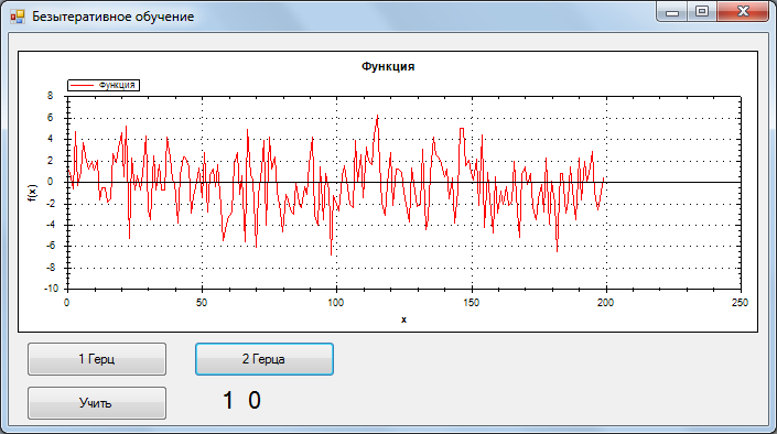
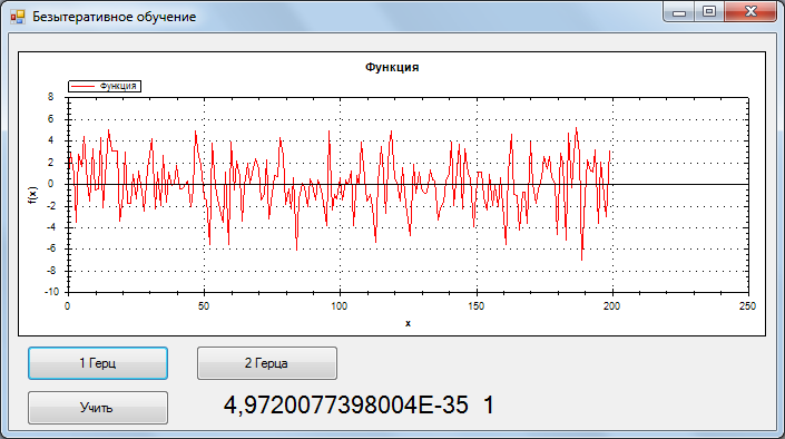
For testing, a training sample of 2 signals without noise, 1 and 2 Hz, 200 counts was taken. One hertz corresponds to the response of the NA {0,1}, two {1.0}.
During testing, the signal + Gaussian noise was recognized. SNR = 0.33
The following is the recognition:
1Hz, the best result

2 Hz, the best result
1 Hz, the worst result
Considering that the accuracy is very high (tested on other signals). I assume that this method reduces the error function to the global minimum.
Learning Code:
In future articles I plan to consider training in multilayer networks, generation of networks with optimal architecture, and training in convolution networks.
In the last article, we looked at the learning method based on the decision of the SLAE, we will not solve it because This is too time consuming process. Now we are interested in this method only vector “B”, this vector reflects how important one or another sign for classification.
\\ B = \ {b_1 ... b_m \}; \\ b_k = - \ sum_ {i = 1} ^ nx_k ^ i \ cdot y ^ i; \\ k \ in [1, m];
\\ B = \ {b_1 ... b_m \}; \\ b_k = - \ sum_ {i = 1} ^ nx_k ^ i \ cdot y ^ i; \\ k \ in [1, m];
And here, because there is an activation f-i with saturation, weights can be expressed as:
\\ W = \ {w_1, ..., w_m \}; \\ W = K \ cdot B;
\\ W = \ {w_1, ..., w_m \}; \\ W = K \ cdot B;
')
The first thing to do is replace yi on ti . Since in the classification problem, “y” can be either 1 (belongs) or 0 (does not belong). That t must be either 1 or -1. From here ti=2 cdotyi−1 . Now
bk=− sumni=1xik cdotti;
Now we will express the coefficient “K” as a fraction, where in the numerator is a function, the inverse of f-activation from 0.99 (it cannot be taken from one because it will be + infinity), and in the denominator the sum of the moduli values of all elements included in the sample use the square root of energy). And all this is multiplied by -1.
The final formula is:
wk= fracf−1a(0.999) cdot sumni=1xik cdotti sumni=1 summj=1|xij|;
For sigmoid, which has the form fa(x)= frac11+exp(− beta cdotx) , reverse f-i - f−1a(x)=− fracln( frac1x−1) beta at beta=1;f−1a(0.99)=$4.
* Small check
Let there be two pairs x ^ 1 = \ {1,0,1,0 \}; y ^ 1 = 1; x ^ 2 = \ {0.7,1,0.1,1 \}; y ^ 2 = 0;x ^ 1 = \ {1,0,1,0 \}; y ^ 1 = 1; x ^ 2 = \ {0.7,1,0.1,1 \}; y ^ 2 = 0; . We calculate the weight according to the formula above:
w1=−1.83;w2=−6.1;w3=5.49;w4=−6.1;
Now let's “run through” our vectors through the resulting neuron, let me remind the neuron response formula:
y(x)=fa( sumni=1wixi);
The first vector gave the result 0.997, the second - 2 cdot10−6 which is very similar to the truth.
*Testing
For testing, a training sample of 2 signals without noise, 1 and 2 Hz, 200 counts was taken. One hertz corresponds to the response of the NA {0,1}, two {1.0}.
During testing, the signal + Gaussian noise was recognized. SNR = 0.33
The following is the recognition:
1Hz, the best result
2 Hz, the best result
1 Hz, the worst result
Considering that the accuracy is very high (tested on other signals). I assume that this method reduces the error function to the global minimum.
Learning Code:
public void Train(Vector[] inp, Vector[] outp) { OutNew = new Vector[outp.Length]; In = new Vector[outp.Length]; Array.Copy(outp, OutNew, outp.Length); Array.Copy(inp, In, inp.Length); for (int i = 0; i < OutNew.Length; i++) { OutNew[i] = 2*OutNew[i]-1; } K = 4.6*inp[0].N*inp.Length; double summ = 0; for (int i = 0; i < inp.Length; i++) { summ += Functions.Summ(MathFunc.abs(In[i])); } K /= summ; Parallel.For(0, _neurons.Length, LoopTrain); } void LoopTrain(int i) { for (int k = 0; k < In[0].N; k++) { for (int j = 0; j < OutNew.Length; j++) { _neurons[i].B.Vecktor[k] += OutNew[j].Vecktor[i]*In[j].Vecktor[k]; } } _neurons[i].W = K*_neurons[i].B; } In future articles I plan to consider training in multilayer networks, generation of networks with optimal architecture, and training in convolution networks.
Source: https://habr.com/ru/post/333382/
All Articles