BFGS method or one of the most effective optimization methods. Python implementation example

The BFGS method, an iterative numerical optimization method, is named after its researchers: B royden, F letcher, G oldfarb, S hanno. It belongs to the class of so-called quasi-Newtonian methods. In contrast to the Newtonian methods, the Hessian functions are not calculated directly in quasi-Newtonian methods, i.e. there is no need to find second order partial derivatives. Instead, the Hessian is calculated approximately from the steps taken before.

There are several modifications of the method:
L-BFGS (limited memory usage) - used in case of a large number of unknowns.
L-BFGS-B is a modification with limited memory usage in a multidimensional cube.
')
The method is efficient and stable, therefore it is often used in optimization functions. For example, in SciPy, a popular library for the python language, in the optimize function, the default is BFGS, L-BFGS-B.

Algorithm

Let some function be given $$$f (x, y)$and we solve the optimization problem: $$$min f (x, y)$.
Where in the general case $$$f (x, y)$is a nonconvex function that has continuous second derivatives.

Step # 1
Initialize the starting point $$$x_0$;
Set the accuracy of the search $$$ε$> 0;
Determine the initial approximation $$$H_0 = B_0 ^ {- 1}$where $$$B_0 ^ {- 1}$- reverse hessian function;

How to choose the initial approximation $$$H_0$?
Unfortunately, there is no general formula that would work well in all cases. As an initial approximation, we can take the Hessian of the function, calculated at the starting point $$$x_0$. Otherwise, a well-conditioned, non-degenerate matrix can be used; in practice, an identity matrix is ​​often taken.

Step 2
We find the point in the direction of which we will perform the search, it is determined as follows:

$$

$$p_k = -H_k * \ nabla f_k$$

Step 3
Calculate $$$x_ {k + 1}$through the recurrence relation:

$$

$$x_ {k + 1} = x_k + α_k * p_k$$

Coefficient $$$α_k$find using linear search (line search), where $$$α_k$satisfies Wolfe conditions :

$$

$$f (x_k + α_k * p_k) \ leq f (x_k) + c_1 * α_k * \ nabla f_k ^ T * p_k$$

$$

$$\ nabla f (x_k + α_k * p_k) ^ T * p_k \ geq c_2 * \ nabla f_k ^ T * p_k$$

Constants $$$s_1$and $$$c_2$choose as follows: $$$0 \ leq c_1 \ leq c_2 \ leq 1$. In most implementations: $$$c_1 = 0.0001$and $$$s_2 = 0.9$.

In fact, we find such $$$α_k$at which the value of the function $$$f (x_k + α_k * p_k)$minimally.

Step 4
Define vectors:

$$

$$s_k = x_ {k + 1} - x_k$$

$$

$$y_k = \ nabla f_ {k + 1} - \ nabla f_k$$

$$$s_k$- algorithm step at iteration, $$$y_k$- gradient change on iteration.

Step number 5
We update the hessian function according to the following formula:

$$

$$H_ {k + 1} = (I - ρ_k * s_k * y_k ^ T) H_k (I - ρ_k * y_k * s_k ^ T) + ρ * s_k * s_k ^ T$$

Where $$$ρ_k$

$$

$$ρ_k = \ frac {1} {y_k ^ T s_k}$$

$$$I$- unit matrix.

Comment

Expression type $$$y_k * s_k ^ T$is the outer product of the two vectors.
Let two vectors be defined $$$U$and $$$V$, then their outer product is equivalent to the matrix product $$$UV ^ T$. For example, for vectors on a plane:

$$

$$UV ^ T = \ begin {pmatrix} U_1 \\ U_2 \ end {pmatrix} \ begin {pmatrix} V_1 & V_2 \ end {pmatrix} = \ begin {pmatrix} U_1V_1 & U_1V_2 \\ U_2V_1 & U_2V_2 \ end {pmatrix }$$

Step 6
The algorithm continues to execute as long as the inequality is true: $$$| \ nabla f_k | > ε$.

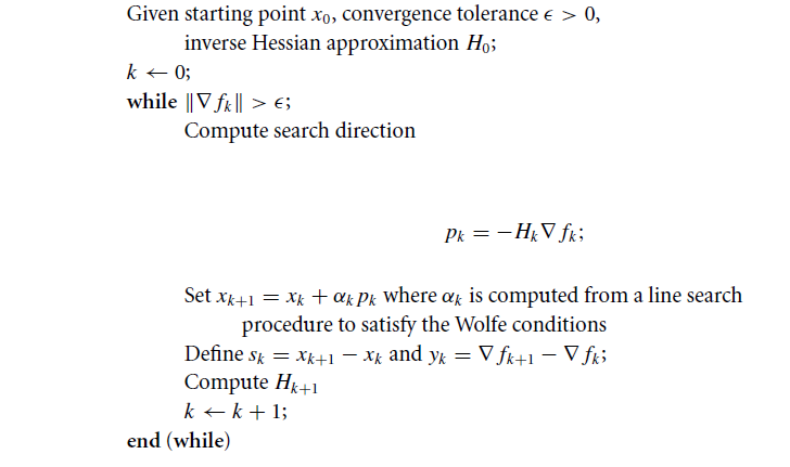
Algorithm schematically

Example

Find the extremum of the following function: $$$f (x, y) = x ^ 2 - xy + y ^ 2 + 9x - 6y + 20$
As a starting point, take $$$x_0 = (1, 1)$;
Accuracy Required $$$ε = 0.001$;

Find the gradient function $$$f (x, y)$:

$$

$$\ nabla f = \ begin {pmatrix} 2x - y + 9 \\ -x + 2y - 6 \ end {pmatrix}$$

Iteration # 0 :

$$

$$x_0 = (1, 1)$$

Find the gradient at the point $$$x_0$:

$$

$$\ nabla f (x_0) = \ begin {pmatrix} 10 \\ -5 \ end {pmatrix}$$

Check on the end of the search:

$$

$$| \ nabla f (x_0) | = \ sqrt {10 ^ 2 + (-5) ^ 2} = $ 11.1$$

$$

$$| \ nabla f (x_0) | = 11.18> 0.001$$

Inequality is not satisfied, so we continue the process of iterations.

Find a point in the direction of which we will search:

$$

$$p_0 = -H_0 * \ nabla f (x_0) = - \ begin {pmatrix} 1 & 0 \\ 0 & 1 \ end {pmatrix} \ begin {pmatrix} 10 \\ -5 \ end {pmatrix} = \ begin {pmatrix} -10 \\ 5 \ end {pmatrix}$$

Where $$$H_0 = I$- unit matrix.

We are looking for this $$$α_0$$$$\ geq$0 to $$$f (x_0 + α_0 * p_0) = min (f (x_0 + α_0 * p_0))$

Analytically, the problem can be reduced to finding the extremum of a function of one variable:

$$$$ display $$ x_0 + α_0 * p_0 = (1, 1) + α_0 (-10, 5) = (1 - 10α_0, 1 + 5α_0) $$ display $$

Then

$$$ inline $ f (α_0) = (1 - 10α_0) ^ 2 - (1 - 10α_0) (1 + 5α_0) + (1 + 5α_0) ^ 2 + 9 (1 - 10α_0) - 6 (1 + 5α_0) + 20 $ inline $

Simplifying the expression, we find the derivative:

$$

$$\ frac {\ partial f} {\ partial x} = 350α_0 - 125 = 0 \ Rightarrow α_0 = 0.357$$

Find the next point $$$x_1$:

$$

$$x_1 = x_0 + α_0 * p_0 = (-2.571, 2.786)$$

$$

$$s_0 = x_1 - x_0 = (-2.571, 2.786) - (1, 1) = (-3.571, 1.786)$$

Calculate the value of the gradient in t. $$$x_1$:

$$

$$\ nabla f (x_1) = \ begin {pmatrix} 1.071 \\ 2.143 \ end {pmatrix}$$

$$

$$y_0 = \ nabla f (x_1) - \ nabla f (x_0) = (1.071, 2.143) - (10, -5) = (-8.929, 7.143)$$

Find the approximation of the Hessian:

$$

$$H_1 = \ begin {pmatrix} 0.694 & 0.367 \ 0.367 & 0.709 \ end {pmatrix}$$

Iteration 1:

$$

$$x_1 = (-2.571, 2.786)$$

$$

$$\ nabla f (x_1) = \ begin {pmatrix} 1.071 \\ 2.143 \ end {pmatrix}$$

Check on the end of the search:

$$

$$| \ nabla f (x_1) | = 2.396> 0.001$$

Inequality is not satisfied, so we continue the iteration process:

$$

$$H_1 = \ begin {pmatrix} 0.694 & 0.367 \ 0.367 & 0.709 \ end {pmatrix}$$

$$

$$p_1 = -H_1 \ nabla f (x_1) = - \ begin {pmatrix} 0.694 & 0.367 \\ 0.367 & 0.709 \ end {pmatrix} \ begin {pmatrix} 1.071 \\ 2.143 \ end {pmatrix} = - \ begin { pmatrix} 1.531 \\ 1.913 \ end {pmatrix}$$

Find $$$α_1$> 0:

$$$ inline $ f (α_1) = -2.296α_1 + (-1.913α_1 + 2.786) ^ 2 - (-1.913α_1 + 2.786) (- 1.531α_1 - 2.571) + (-1.531α_1 - 2.571) ^ 2 - 19.86 $ inline $

$$

$$\ frac {\ partial f} {\ partial α_1} = 6.15α_1 - 5.74 = 0 \ Rightarrow α_1 = 0.933$$

Then:

$$

$$x_2 = (-3.571, 0.786)$$

$$

$$s_1 = x_2 - x_1 = (-4, 1) - (-2.571, 2.786) = (-1.429, -1.786)$$

Calculate the value of the gradient at $$$x_2$:

$$

$$\ nabla f (x_2) = \ begin {pmatrix} 0 \\ 0 \ end {pmatrix}$$

$$

$$g_1 = \ nabla f (x_2) - \ nabla f (x_1) = (0, 0) - (1.071, 2.143) = (-1.071, -2.143)$$

$$

$$H_2 = \ begin {pmatrix} 0.667 & 0.333 \ 0.333 & 0.667 \ end {pmatrix}$$

Iteration 2 :

$$

$$x_2 = (-4, 1)$$

Check on the end of the search:

$$

$$| \ nabla f (x_2) | = 0 <0.001$$

Inequality is performed hence the search ends. Analytically we find the extremum of the function; it is reached at the point $$$x_2$.

More about the method

Each iteration can be performed with a cost $$$O (n ^ 2)$(plus the cost of the function calculation and the gradient estimate). There is no $$$O (n ^ 3)$operations such as solving linear systems or complex mathematical operations. The algorithm is stable and has superlinear convergence, which is sufficient for most practical problems. Even if Newton's methods converge much faster (quadratically), the cost of each iteration is higher, since it is necessary to solve linear systems. An undeniable advantage of the algorithm, of course, is that there is no need to calculate the second derivatives.

Very little is theoretically known about the convergence of the algorithm for the case of a non-convex smooth function, although it is generally accepted that the method works well in practice.

The BFGS formula has self-correcting properties. If matrix $$$H$does not correctly evaluate the curvature of the function, and if this poor estimate slows down the algorithm, then the Hessian approximation tends to correct the situation in a few steps. Self-correcting properties of the algorithm work only if the corresponding linear search is implemented (the conditions of Wolfe are met).

Python implementation example

The algorithm is implemented using the numpy and scipy libraries. Linear search was implemented by using the line_search () function from the scipy.optimize module. The example imposes a limit on the number of iterations.

''' Pure Python/Numpy implementation of the BFGS algorithm. Reference: https://en.wikipedia.org/wiki/Broyden%E2%80%93Fletcher%E2%80%93Goldfarb%E2%80%93Shanno_algorithm ''' #!/usr/bin/python # -*- coding: utf-8 -*- import numpy as np import numpy.linalg as ln import scipy as sp import scipy.optimize # Objective function def f(x): return x[0]**2 - x[0]*x[1] + x[1]**2 + 9*x[0] - 6*x[1] + 20 # Derivative def f1(x): return np.array([2 * x[0] - x[1] + 9, -x[0] + 2*x[1] - 6]) def bfgs_method(f, fprime, x0, maxiter=None, epsi=10e-3): """ Minimize a function func using the BFGS algorithm. Parameters ---------- func : f(x) Function to minimise. x0 : ndarray Initial guess. fprime : fprime(x) The gradient of `func`. """ if maxiter is None: maxiter = len(x0) * 200 # initial values k = 0 gfk = fprime(x0) N = len(x0) # Set the Identity matrix I. I = np.eye(N, dtype=int) Hk = I xk = x0 while ln.norm(gfk) > epsi and k < maxiter: # pk - direction of search pk = -np.dot(Hk, gfk) # Line search constants for the Wolfe conditions. # Repeating the line search # line_search returns not only alpha # but only this value is interesting for us line_search = sp.optimize.line_search(f, f1, xk, pk) alpha_k = line_search[0] xkp1 = xk + alpha_k * pk sk = xkp1 - xk xk = xkp1 gfkp1 = fprime(xkp1) yk = gfkp1 - gfk gfk = gfkp1 k += 1 ro = 1.0 / (np.dot(yk, sk)) A1 = I - ro * sk[:, np.newaxis] * yk[np.newaxis, :] A2 = I - ro * yk[:, np.newaxis] * sk[np.newaxis, :] Hk = np.dot(A1, np.dot(Hk, A2)) + (ro * sk[:, np.newaxis] * sk[np.newaxis, :]) return (xk, k) result, k = bfgs_method(f, f1, np.array([1, 1])) print('Result of BFGS method:') print('Final Result (best point): %s' % (result)) print('Iteration Count: %s' % (k)) 

Thank you for your interest in my article. I hope she was useful to you and you have learned a lot.

With you was FUNNYDMAN. Bye everyone!